This lesson has two sections. First demonstrates a method to simulate one-participant data. The function, simulate, in the ggdmc package creates a data frame based on the parameter vector and the model (both are defined by a user) with nsim observations for each row in model. ps is the true parameter vector.
Second section shows a method to conduct a process model. Specifically, the section conducts a simulation experiment to describe the British tea example on p 37 in Maxwell & Delaney (2004). See Maxwell and Delaney (2004) for an analytic method to calculate the same probabilities. Here I directly model the Britich tea example, approximating the same probabilities. The analytic method is just to use a binominal distribution and the idea of combinations and permutations.
One-participant simulation
This line define one S (stimulus) factor with two levels. So this model defines one two experimental conditions.
factors = list(S = c(“s1”, “s2”)),
Below are the R codes for defining a model and for simulating data from the model.
require(ggdmc)
model <- BuildModel(
   p.map     = list(A = "1", B = "R", t0 = "1", mean_v = "M", sd_v = "M", st0 = "1"),
   match.map = list(M = list(s1 = "r1", s2 = "r2")),
   factors   = list(S = c("s1", "s2")),  ## one factor with two levels, so only
   constants = c(sd_v.false = 1, st0 = 0),
   responses = c("r1", "r2"),
   type      = "norm")

p.vector <- c(A = .75, B.r1 = .25, B.r2 = .15, t0 = .2, mean_v.true = 2.5,
               mean_v.false = 1.5, sd_v.true = 0.5)
This just is to simulate only one observation per condition to check the function.
set.seed(123)  ## Set seed to get the same simulation
dat <- simulate(model, nsim = 1, ps = p.vector)
##    S  R        RT
## 1 s1 r1 0.3327392
## 2 s2 r1 0.3797985
The following simulates 500 observations per condition. So in total, there are 1000 observations.
ntrial <- 5e2  ## number of trials per condition
dat <- simulate(model, nsim = ntrial, ps = p.vector)
dplyr::tbl_df(dat)
##  A tibble: 1,000 x 3
##    S     R        RT
##    <fct> <fct> <dbl>
##  1 s1    r2    0.533
##  2 s1    r2    0.494
##  3 s1    r1    0.497
##  4 s1    r2    0.310
##  5 s1    r1    0.462
##  6 s1    r2    0.345
##  7 s1    r2    0.430
##  8 s1    r1    0.384
##  9 s1    r2    0.310
## 10 s1    r1    0.302
# # ... with 990 more rows
Note that model and data are in fact two separate objects. To fit data with certain models, we need to bind them together with BuildDMI. This is useful to facilitate model comparison. That is, a data set can bind with many different models, so we can compare them to see which model may fit the data better so perhaps provide a better account. I used a term, data-model instance (dmi), coined by Matthew Gretton.
dmi <- BuildDMI(dat, model)
We can the codes introduced in the “Descriptive Statistics” to check the correct 10%, 50%, 90% quantile RTs and accuracy, separately, for each level of the stimulus factor.
First I convert the dmi data frame to a data table and then create a new accuracy (logical) column, C.
require(data.table)
d <- data.table(dmi)
d$C <- ifelse(d$S == "s1" & d$R == "r1", TRUE,
       ifelse(d$S == "s2" & d$R == "r2", TRUE,
       ifelse(d$S == "s1" & d$R == "r2", FALSE,
       ifelse(d$S == "s2" & d$R == "r1", FALSE, NA))))

d[, .(q1 = round(quantile(RT, .1), 2),
      q5 = round(quantile(RT, .5), 2),
      q9 = round(quantile(RT, .9), 2)), .(C, S)]
##        C  S   q1   q5   q9
## 1:  TRUE s1 0.32 0.42 0.56
## 2:  TRUE s2 0.28 0.39 0.52
## 3: FALSE s1 0.27 0.37 0.50
## 4: FALSE s2 0.32 0.39 0.54

pro <- d[, .N, .(C, S)]
pro[, NN := sum(N), .(S)]
pro[, value := N/NN]
cp <- pro[C == TRUE] ## correct percentage
##       C  S   N  NN value
## 1: TRUE s1 333 500 0.666
## 2: TRUE s2 391 500 0.782

ep <- pro[C == FALSE] ## error percentage
##        C  S   N  NN value
## 1: FALSE s1 167 500 0.334
## 2: FALSE s2 109 500 0.218
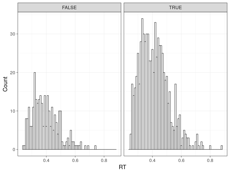
Plot the RT distributions
require(ggplot2)
bw <- .01 ## 10 ms binwidth
p0 <- ggplot(d, aes(RT)) +
      geom_histogram(binwidth = bw, fill = "white", colour = "black") +
      facet_grid(.~C) +
      theme_bw(base_size = 18)
print(p0)
British tea example
This section shows how we may test an hypothetical question directly via a simulation. Quoted from Maxwell and Delaney (p. 37, 2004)
“A lady declares that by tasting a cup of tea made with milk, she can discriminate whether the milk or the tea infusion was first added to the cup. We will consider the problem of designing an experiment by means of which this assertion can be tested. (Fisher, 1935/1971, p. 11)”
This is essential a binominal decision making. That is, the decision maker (“the lady”) in question will be presented one cup of tea after another and then her task is to decide if the cup is made by milk or tea is added first.
This following function, British.tea implements a process model to describe the above “British tea example”. That is, it conducts a simulation experiment of presenting 8 (i.e., n) cups of tea to a participant. The n equals 8 is decided arbitrarily here.
One additional information (i.e., assumption) is that the participant is told half of the cups are milk first and tea and vice versa. So when simulating the chance only scenario, we need also to take this into consideration. That is, after making a decision for a cup (either MT or TM), the (chance) probability state should adjust accordingly.
##' British tea example
##'
##' The function runs a simulation study to test the British tea example
##'
##' @param the number of observation (cups of tea)
##' @param correct correct sequence: First four cups are tea and milk
##  (TM = 1), the next four cups are milk and then tea (MT = 0).
##' @param verbose print more information
##'
##' @export
British.tea <- function(n = 8, correct = c(1,1,1,1, 0,0,0,0),
                        verbose = TRUE) {

    MT <- n/2 ## 0 indicates milk and then tea (MT)
    TM <- n/2 ## 1 indicates tea and then milk (TM)

    ## Create three containers
    ## 1. x0 is a "n x 2" matrix to store the evolution of chance probabilities
    ## 2. res is a n-element numeric vector
    ## 3. acc is a n logical vector; default value is FALSE
    x0 <- matrix(numeric(n*2), ncol = 2)
    res <- numeric(n)
    acc <- rep(FALSE, n)

    ## Begin the experiment, presenting one cup after another
    for (i in 1:n) {
        if (verbose) cat("Cup", i, "in total", sum(MT, TM), " cup(s)\n")

		## store the chance probabilities of MT and TM in probs
        probs <- c(MT / (MT + TM), TM / (MT + TM))
        if (verbose) cat("Chances probabilities of (MT, TM): ", probs, "\n")

        x0[i, ] <- probs
        decision <- sample(c(0, 1), 1, prob = probs);
         if (decision == 0) {
             if (verbose) cat("This cup is made by adding milk first\n")
             MT <- MT - 1
             res[i] <- decision
             if (decision == correct[i]) acc[i] <- TRUE
         } else if (decision == 1) {
             if (verbose) cat("This cup is made by adding tea first\n")
             TM <- TM - 1
             res[i] <- decision
             if (decision == correct[i]) acc[i] <- TRUE
         } else cat("Unexpected situation\n")

         if (verbose) cat("Current state", i, ": ", c(MT, TM), "\n\n")
    }
    if (verbose) cat("Done\n")
    return(list(x0, res, correct, acc))
}
The simulation starts from the for loop.
for (i in 1:n) {…}
The for loop presents a cup of tea after another until the nth cup. Before the participant make a decision, the chance probabilities of the two possible outcomes are stored in x0 variable.
probs <- c(probMT, probTM)
x0[i, ] <- probs
And then the sample function acts as a chance mechanism to simulate the participant’s (chance) decision making process.
decision <- sample(c(0, 1), 1, replace = TRUE, prob = probs);
The function randomly choose two numbers, c(0, 1), with the probabilities, probs to for the first and second number.
    ## Begin the experiment, presenting one cup after another
    for (i in 1:n) {
        if (verbose) cat("Cup", i, "in total", sum(MT, TM), " cup(s)\n")

        probMT <- MT / (MT + TM)   ## chance probability of MT 0
        probTM <- TM / (MT + TM)   ## chance probability of TM 1
        probs  <- c(probMT, probTM)

        if (verbose) cat("Chances probabilities of (MT, TM): ", probs, "\n")

        x0[i, ] <- probs
        decision <- sample(c(0, 1), 1, prob = probs);

         if (decision == 0) {
             if (verbose) cat("This cup is made by adding milk first\n")
             MT <- MT - 1
             res[i] <- decision
             if (decision == correct[i]) acc[i] <- TRUE
         } else if (decision == 1) {
             if (verbose) cat("This cup is made by adding tea first\n")
             TM <- TM - 1
             res[i] <- decision
             if (decision == correct[i]) acc[i] <- TRUE
         } else cat("Unexpected situation\n")

         if (verbose) cat("Current state", i, ": ", c(MT, TM), "\n\n")
}
Conduct one experiment and print information
ncup <- 8
cor <- c(rep(1, 4), rep(0, 4));
res <- British.tea(ncup, cor, TRUE)
Cup 1 in total 8 cup(s).
Chances probabilities of (MT, TM): 0.5 0.5 This cup is made by adding tea first Current state 1 : 4 3
Cup 2 in total 7 cup(s).
Chances probabilities of (MT, TM): 0.5714286 0.4285714 This cup is made by adding milk first Current state 2 : 3 3
Cup 3 in total 6 cup(s).
Chances probabilities of (MT, TM): 0.5 0.5 This cup is made by adding tea first Current state 3 : 3 2
Cup 4 in total 5 cup(s).
Chances probabilities of (MT, TM): 0.6 0.4 This cup is made by adding milk first Current state 4 : 2 2
Cup 5 in total 4 cup(s).
Chances probabilities of (MT, TM): 0.5 0.5 This cup is made by adding milk first Current state 5 : 1 2
Cup 6 in total 3 cup(s).
Chances probabilities of (MT, TM): 0.3333333 0.6666667 This cup is made by adding tea first Current state 6 : 1 1
Cup 7 in total 2 cup(s).
Chances probabilities of (MT, TM): 0.5 0.5 This cup is made by adding tea first Current state 7 : 1 0
Cup 8 in total 1 cup(s).
Chances probabilities of (MT, TM): 1 0 This cup is made by adding milk first Current state 8 : 0 0
Done
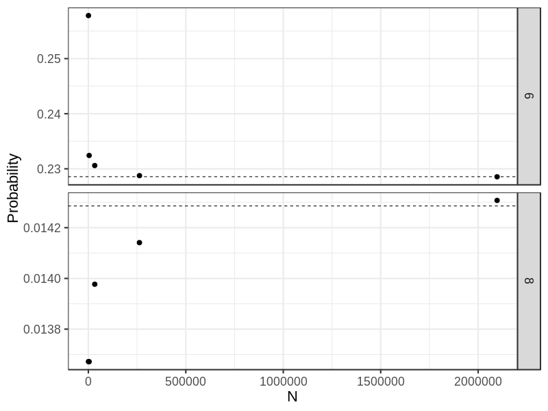
Now I replicate the experiments separately for 512, 4096, 32768, 262144, and 2097152 times and store each result in a list, called exp.
n <- 8^(3:7);
exp <- vector("list", length(n))

## Use parallel package to conduct experiments
## 100.636 s
library(parallel)
cl <- makeCluster(detectCores())
clusterExport(cl, c("British.tea", "ncup", "cor"))
system.time(
    for (i in 1:length(n)) {
        exp[[i]] <- parSapply(cl, 1:n[i], function(i, ...) {British.tea(ncup, cor, FALSE)} )
    }
)
stopCluster(cl)
## Without using parallel
## for(i in 1:length(n)) {
##     exp[[i]] <- replicate(n[i], British.tea(ncup, cor, FALSE))
## }

res3 <- numeric(length(n)); res3  ## to store the result when 6 corrects
res4 <- numeric(length(n)); res4  ## to store the result when 8 corrects

## Collect results
for(i in 1:length(n)) {
    c3 <- 0
    c4 <- 0
    for(j in 1:n[i]) {
         ## Calculate exactly 4 corrects
         if(all(exp[[i]][,j][[4]])) c4 <- c4 + 1
         if(sum(exp[[i]][,j][[4]]) == 6) c3 <- c3 + 1
    }
    res3[i] <- c3 / n[i]
    res4[i] <- c4 / n[i]
}


round(res3, 4) ## [1] 0.2578 0.2324 0.2306 0.2288 0.2286
round(res4, 4) ## [1] 0.0137 0.0137 0.0140 0.0141 0.0143
require(ggplot2); require(data.table)
## Plot the result
## (How to add differernt horizontal lines on each facet)
DT <- data.table(x= rep(n, 2), y = c(res3, res4), gp = rep(c("6", "8"), each = 5),
                 ref = rep(c(16/70, 1/70), each = 5))

## Dashlines show theoretically probabilities
p0 <- ggplot(DT, aes(x, y)) +
    geom_point(size = 3) +
    geom_hline(aes(yintercept = ref), linetype = "dashed") +
    ## scale_x_log10(name = "N") +
    xlab("N") + ylab("Probability") +
    facet_grid(gp~., scales = "free") +
    theme_bw(base_size = 22)

print(p0)