Disclaimer: This is part of our power analysis for a series of experiments for driving, traffic, and driving-simulator tasks. The note documented our the implementation details of the simulation and analysis plans.

In these would-be traffic / driving tasks, participants will be making decisions on whether to cross streets or driving through an intersection within a time limit, e.g., 3 seconds. Thus, they will face tasks belonging to the category of one-choice task, where people decide to commit a response or abort. The latter will result in a RT over the time limit, e.g., 3 seconds.

To model such tasks, using a diffusion model, one could opt for the Wald, aka inverse Gaussian, distribution, where one can find an explicit solution for the distribution of RTs. “However, there is no explicit mathematical solution for a RT distribution with negative drift rate. Negative drift rates are produced from the left tail of the across-trial distribution of drift rates” (Ratcliff, 2015). That is, if we also want to also use between-trial drift rate variability, we have to seek alternative solution.

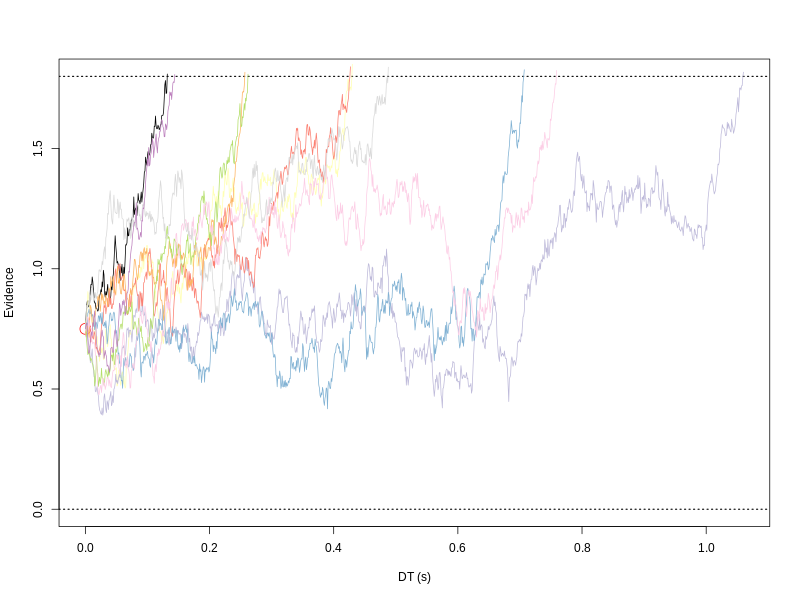
In the following, I opt for a similar solution as in Ratcliff (2015), using a random walk approximation. Differing from what he did, in the following simulation, I fixed the z, s and t0.

require(subplex)
Rcpp::sourceCpp("r1d.cpp")

objective_fun <- function(par, data, tmax, h, nsim) {
    pvec <- c(par[1:2], .75, 0, 1)

    tmp <- r1c(nsim, pvec, tmax, h)
    
    tmp <- tmp[!is.na(tmp[,2]), ]
    tmp <- tmp[!is.na(tmp[,1]), ]
    
    over_tmax <- tmp[,2] == tmax
    sim <- tmp[!over_tmax, ]
    pred_RT <- sim[,1]

    if (length(pred_RT) == 0) {
        error <- 1e9
    } else {
        data_RT <- data[,1]
        pred_q0 <- quantile(pred_RT, probs = seq(.1, .9, .2))
        data_q0 <- quantile(data_RT, probs = seq(.1, .9, .2))
        error <- sum( (data_q0 - pred_q0)^2 / mymean(data_q0, 1)^2 )
    }
  return(error)
}

## A normalization constant; may not needed
mymean <- function(x=NULL, nozero=0)
{
    if(is.null(x)) {
      out <- 1
    } else {
      out <- ifelse(mean(x)==0 && nozero, 1, mean(x))
    }
    return(out)
}

A Recovery Study

Following Ratcliff (2015), I assumed an upper time limit at 3 seconds. The target “true” parameters are: v = 2.35, a = 1.8. The start point, non-decision time, and within-trial standard deviation were fixed at 0.75, 0 and 1. I used 20,000 iterations to approximate the process.

tmax <- 3
h <- 1e-3   ## Ratcliff's used 0.5 ms
n <- 1e3    ## Assumed number of data points
p.vector <- c(v=2.35, a=1.8, z=.75, t0=0, s=1)  ## True values
nsim <- 2e4 ## Using Ratcliff's iteration number

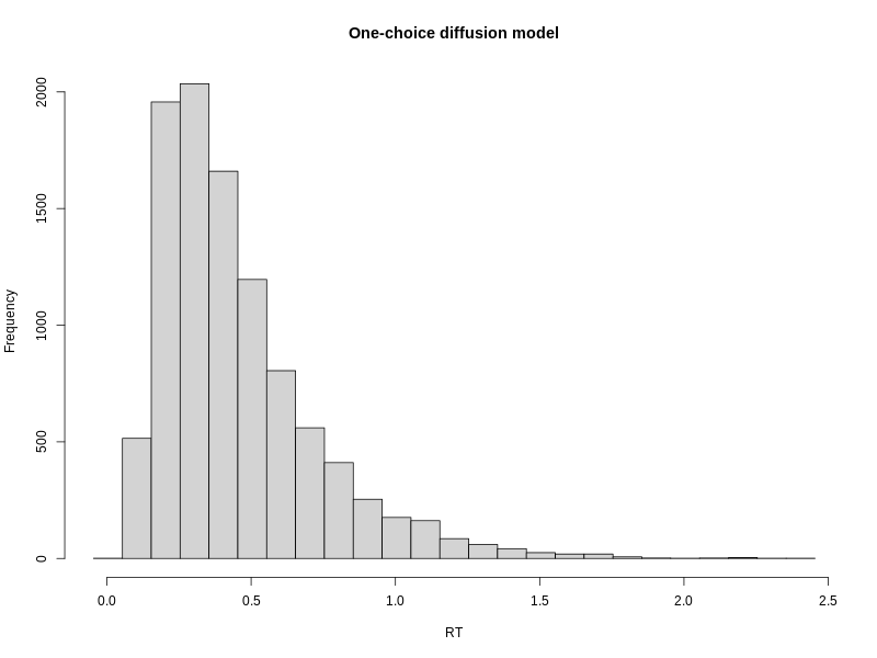
First I simulated a “true” data set as the target to recover. This particular set of “true” parameters behaved well, so it rarely produced RT over 3 seconds.

tmp <- r1c(n, p.vector, tmax, h)
tmp <- tmp[!is.na(tmp[,2]), ]
tmp <- tmp[!is.na(tmp[,1]), ]
over_tmax <- tmp[,2] == tmax

sum(over_tmax)
sim <- tmp[!over_tmax, ]

Then I used subplex to estimate the two target parameters, v = 2.35 and a = 1.8.

fit <- subplex(par = runif(2), fn = objective_fun, hessian = FALSE,
               data = sim, tmax=tmax, h=h, nsim=nsim)

The estimations are v = 2.62 and a = 1.9. Both are very close to true values.

str(fit)
## List of 6
##  $ par        : num [1:2] 2.62 1.9
##  $ value      : num 0.000371
##  $ counts     : int 352
##  $ convergence: int 0
##  $ message    : chr "success! tolerance satisfied"
##  $ hessian    : NULL
str(fit)

Next

1. Task 1 is to conduct a 100 resampling recover studies to investigate the variability.
2. Task 2 is to decrease the trial number to perhaps 100 or 200 to see the impact of using low trial number.
3. Task 3 is to examine the two typical manipulation, task difficulty and speed-accuracy tradeoff to see how the estimate parameters reflect the influence and whether the trial number and the participant number are enough to detect any effects.
4. Task 4 is to add collapsing bound mechanism.

## parameters <- parallel::mclapply(1:100, function(i) 
##               try(doit(p.vector, n, tmax, h, nsim), TRUE),
##               mc.cores = getOption("mc.cores", ncore))
## 

Reference

Ratcliff, R. Modeling one-choice and two-choice driving tasks. Atten Percept Psychophys 77, 2134–2144 (2015). https://doi.org/10.3758/s13414-015-0911-8