In this tutorial, I used the DE-MCMC sampler (Turner et al., 2013) to fit a hierarchical LBA model. This particular design has a stimulus (S) and a frequency (F) factor.
Set-up Model
I used the usual DMC-style syntax to set up the model. I hope, at this point, it might be clear for the reader who has read through the Model Array, that the meaning of syntax in p.map.
p.map = list(A = “1”, B = “R”, t0 = “1”, mean_v = c(“F”, “M”), sd_v = “M”, st0 = “1”),
library(ggdmc)

model <- BuildModel(
          p.map = list(A = "1", B = "R", t0 = "1",
                    mean_v = c("F", "M"), sd_v = "M", st0 = "1"),
          match.map = list(M = list(s1=1, s2=2)),
          factors   = list(S = c("s1", "s2"),F = c("f1", "f2")),
          constants = c(sd_v.false = 1, st0 = 0),
          responses = c("r1", "r2"),
          type      = "norm")
## Parameter vector names (unordered) are: ( see attr(,"p.vector") )
## [1] "A"               "B.r1"            "B.r2"            "t0"
## [5] "mean_v.f1.true"  "mean_v.f2.true"  "mean_v.f1.false" "mean_v.f2.false"
## [9] "sd_v.true"
##
## Constants are (see attr(,"constants") ):
## sd_v.false        st0
##          1          0
##
## Model type = norm (posdrift = TRUE )

npar <- length(GetPNames(model))
mean_v = c(“F”, “M”), refers to that the mean of the drift rate is affected by the F and M factors. The former is an experimental factor and the latter is a latent LBA specific factor. B = “R” refers to that the travel distance parameter is affected by the response factor, which in a binary decision task, is two levels. Here it is either “r1” or “r2”, defined in the response option / argument.
responses = c(“r1”, “r2”),
Therefore, the data.frame (an R way to store real or simulated data ) should have an R column, similar to the below:
> dplyr::tbl_df(dat)
# A tibble: 40,000 x 5
   s     S     F     R        RT
   <fct> <fct> <fct> <fct> <dbl>
 1 1     s1    f1    r1    0.745
 2 1     s1    f1    r1    0.883
 3 1     s1    f1    r1    0.884
 4 1     s1    f1    r1    0.678
 5 1     s1    f1    r1    0.729
 6 1     s1    f1    r1    0.803
 7 1     s1    f1    r1    0.735
 8 1     s1    f1    r1    0.756
 9 1     s1    f1    r1    0.847
10 1     s1    f1    r1    0.855
# ... with 39,990 more rows
- s refers to subject label,
- S is stimulus factor,
- F is frequency factor,
- R is response factor,
- fct refers to factor, namely a categorical variable,
- dbl refers to double, namely a continuous, numerical variable.
In this design, the S factor does not affect any model parameters, and the F factor affects the mean of the drift rate, mean_v = c(“F”, “M”). Because this is a parameter recovery study, I simulated a data set based on the above model. Similarly, I used a random-effects model to generate the data set, so I defined a set of population distribution for each LBA parameters. The names of the parameter were reported by the BuildModel function.
Simulate Data
pop.mean <- c(A=.4, B.r1=.6, B.r2=.8, t0=.3, mean_v.f1.true=1.5,
              mean_v.f2.true=1, mean_v.f1.false=0, mean_v.f2.false=0,
              sd_v.true = .25)
pop.scale <-c( rep(.1, 3), .05, rep(.2, 4), .1)
names(pop.scale) <- names(pop.mean)

pop.prior <- BuildPrior(
  dists = rep("tnorm", npar),
  p1    = pop.mean,
  p2    = pop.scale,
  lower = c(rep(0, 3), .1, rep(NA, 4), 0),
  upper = c(rep(NA, 3), 1, rep(NA, 5)))

dat <- simulate(model, nsim = 30, nsub = 40, prior = pop.prior)
dmi <- BuildDMI(dat, model)
ps <- attr(dat, "parameters")
Then I set up prior distributions and hyper-prior distributions.
### FIT RANDOM EFFECTS
p.prior <- BuildPrior(
  dists = rep("tnorm", npar),
  p1    = pop.mean,
  p2    = pop.scale*5,
  lower = c(0,0,0,.1,NA,NA,NA,NA,0),
  upper = c(NA,NA,NA,NA,NA,NA,NA,NA,NA))
mu.prior <- BuildPrior(
  dists = rep("tnorm", npar),
  p1    = pop.mean,
  p2    = c(1,1,1,1,2,2,2,2,1),
  lower = c(0,0,0,.1,NA,NA,NA,NA,0),
  upper = c(NA,NA,NA,NA,NA,NA,NA,NA,NA))

sigma.prior <- BuildPrior(
  dists = rep("beta", npar),
  p1    = c(A=1, B.r1=1, B.r2=1, t0=1, mean_v.f1.true=1,
            mean_v.f2.true=1, mean_v.f1.false=1, mean_v.f2.false=1,
            sd_v.true = 1),
  p2    = rep(1, npar))

###### Must names "pprior", "location", and "scale" to the prirors list  #######
priors <- list(pprior=p.prior, location=mu.prior, scale=sigma.prior)
###### Must names "pprior", "location", and "scale" to the prirors list  #######
Sampling
Next, I started the sampling. When the debug argument is set TRUE, the run function uses the conventional DE-MCMC sampler, with the its original migration operator.
fit0 <- StartNewsamples(dmi, priors)
fit  <- run(fit0, thin = 8)
Model Diagnosis
Next, I checked if the model has converged and analyze the model estimation. In this tutorial, I did the numerical checks firstly by calculating the potential scale reduction factors (Brook & Gelman,1998). All are less than 1.05, suggesting all chains are well mixed.
rhat <- hgelman(fit, verbose = TRUE)
## hyper     1     2     3     4     5     6     7     8     9    10    11    12    13
##  1.02  1.01  1.01  1.01  1.01  1.01  1.01  1.01  1.01  1.01  1.01  1.01  1.01  1.01
##    14    15    16    17    18    19    20    21    22    23    24    25    26    27
##  1.01  1.01  1.01  1.01  1.01  1.01  1.01  1.01  1.01  1.01  1.01  1.01  1.01  1.01
##    28    29    30    31    32    33    34    35    36    37    38    39    40
##  1.01  1.01  1.01  1.01  1.01  1.01  1.01  1.01  1.01  1.01  1.01  1.01  1.01
Then, I calculated effective samples at the hyper parameters, for one participant at the parameter of the data level, and similarly for all participants. This is to check if enough posterior samples are drawn.
hes <- effectiveSize(hsam, hyper = TRUE)
##
##               A.h1            B.r1.h1            B.r2.h1              t0.h1
##               4655               1416               1152               2061
##  mean_v.f1.true.h1  mean_v.f2.true.h1 mean_v.f1.false.h1 mean_v.f2.false.h1
##               1748               2828               1504               1505
##       sd_v.true.h1               A.h2            B.r1.h2            B.r2.h2
##               3997               3406               3611               2630
##              t0.h2  mean_v.f1.true.h2  mean_v.f2.true.h2 mean_v.f1.false.h2
##               4906               5329               4615               4342
## mean_v.f2.false.h2       sd_v.true.h2
##               4481               3887

es1 <- effectiveSize(hsam[[1]])
##               A            B.r1            B.r2              t0  mean_v.f1.true
##           13531            2819            2629            6100            3755
##  mean_v.f2.true mean_v.f1.false mean_v.f2.false       sd_v.true
##            3793            4983            4239            6572

es <- effectiveSize(hsam)
round(apply(data.frame(es), 1, mean))
round(apply(data.frame(es), 1, sd))
round(apply(data.frame(es), 1, max))
round(apply(data.frame(es), 1, min))
##               A            B.r1            B.r2              t0  mean_v.f1.true
## Mean      11159            2972            2726            6577            4055
## SD         2728             295             172             903             562
## MAX       13967            3778            3196            8183            5273
## MIN        4525            2382            2331            4581            3092
##  mean_v.f2.true mean_v.f1.false mean_v.f2.false       sd_v.true
##            3654            4793            4683            8110
##             598             435             455            1748
##            5056            5582            5699           13163
##            2647            3960            3865            5830
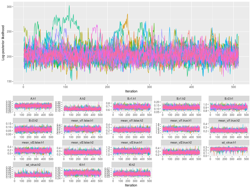
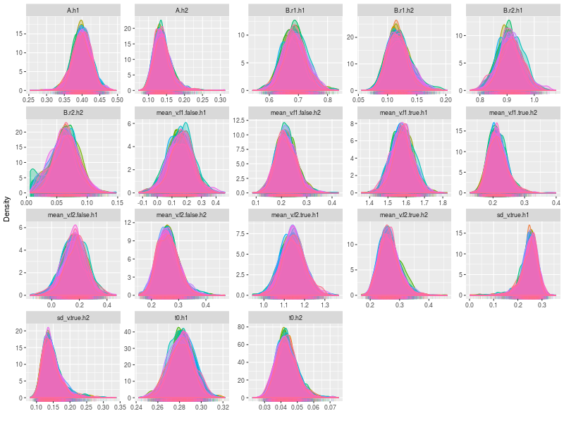
Then I did the visual check by plotting the six types of trace and density plots. Firstly, I plot the hyper parameters. By entering TRUE to the option, save, you save the data in a data.table format1, for further processing. For instance, you can change the figure to fit the publication requirement.
- Trace plots of posterior log-likelihood at hyper level
- Trace plots of the hyper parameters
- Posterior density plots the hyper parameters
plot(hsam, hyper = TRUE)
DT1 <- plot(hsam, hyper = TRUE, pll = FALSE, save = TRUE)
plot(hsam, hyper = TRUE, pll = FALSE, den = TRUE)
Next I checked the trace plots of the posterior log-likelihood and each of the LBA parameters at the data level.
- Trace plots of posterior log-likelihood at the data level
- Trace plots of the LBA parameters for each participants
plot(hsam)
plot(hsam, pll = FALSE)
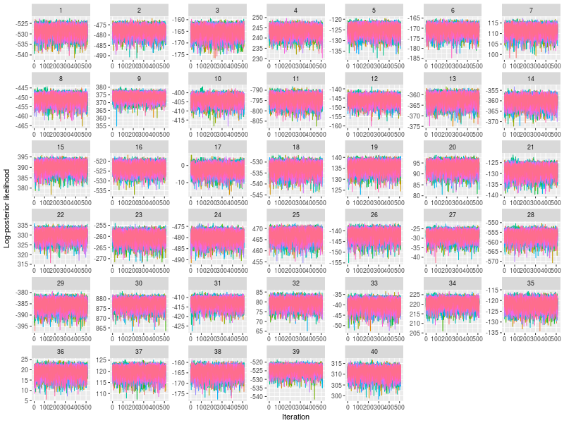
Last, I checked the (posterior) density plots at the data level. There are too many density plots for each participants (nsubject x nparameter = 360), so I did not present them here.
- Posterior density plots the LBA parameters for each parameters
Because this is a parameter recovery study, in the following, I used summary function to check whether Bayesian estimates do recover the true parameters of all participant as well as the mechanism of data generation, namely, pop.mean and pop.scale.
There are five arguments in the summary function you need to know to trigger the smart parameter recovery computation. First is hyper = TRUE, which calculate the phi array / matrix, which stores hyper parameters. Second is the recovery = TRUE, which informs the function to look for a true parameter vector, which you should enter it at ps argument (ps = pop.mean). Otherwise, the function will throw an error message, complaining that it cannot find the true parameter vector.
est1 <- summary(hsam, hyper = TRUE, recovery = TRUE, ps = pop.mean, type = 1)
## Error in summary_recoverone(samples, start, end, ps, digits, verbose) :
## Names of p.vector do not match parameter names in samples
The fourth argument is type = 1. This is a hyper parameter recovery specific. This is to recover the location (mostly mean) parameters. When type = 2, the function will attempt to recover the scale parameters, which mostly refer to standard deviations. The last useful argument is verbose = TRUE, printing message.
est1 <- summary(hsam, hyper = TRUE, recovery = TRUE, ps = pop.mean, type = 1)
## No print, the estimates are stored in est1.

est2 <- summary(hsam, hyper = TRUE, recovery = TRUE, ps = pop.scale, type = 2,
verbose = TRUE)
## Storing estmates in est2 and print results rounding to the second digits
##                   A B.r1  B.r2 mean_v.f1.false mean_v.f1.true mean_v.f2.false
## True           0.10 0.10  0.10            0.20           0.20            0.20
## 2.5% Estimate  0.10 0.09  0.02            0.15           0.17            0.19
## 50% Estimate   0.14 0.12  0.06            0.22           0.21            0.26
## 97.5% Estimate 0.19 0.16  0.10            0.30           0.27            0.34
## Median-True    0.04 0.02 -0.04            0.02           0.01            0.06
##                mean_v.f2.true sd_v.true    t0
## True                     0.20      0.10  0.05
## 2.5% Estimate            0.21      0.11  0.03
## 50% Estimate             0.26      0.14  0.04
## 97.5% Estimate           0.34      0.21  0.06
## Median-True              0.06      0.04 -0.01
By checking the Median-True, namely 50% quantile minus true values, I can confirm that I did recover the true hyper scale parameters. The lines, 2.5% Estimate and 97.5% Estimate inform that the 95% credible intervals, cover the true hyper parameters well. As expected the A and B parameters are sometimes at the boundaries of the 95% intervals, as they are linearly correlated.
More often, researchers concern the location estimates, which I printed out the results stored in est1.
                  A B.r1 B.r2 mean_v.f1.false mean_v.f1.true mean_v.f2.false
True           0.40 0.60 0.80            0.00           1.50            0.00
2.5% Estimate  0.35 0.61 0.83            0.00           1.47            0.00
50% Estimate   0.40 0.68 0.91            0.16           1.58            0.17
97.5% Estimate 0.45 0.76 0.99            0.31           1.68            0.32
Median-True    0.00 0.08 0.11            0.16           0.08            0.17
               mean_v.f2.true sd_v.true    t0
True                     1.00      0.25  0.30
2.5% Estimate            1.04      0.17  0.26
50% Estimate             1.14      0.25  0.28
97.5% Estimate           1.25      0.30  0.30
Median-True              0.14      0.00 -0.02
The estimates look pretty good. My estimation correctly reflects the difference of the two threshold-related parameters. The true values are B.r1 = .6 and _B.r2 = .8. The estimates are B.r1 = .68 and _B.r2 = .91 (B.r2 > B.r1). Even the difference is very close (0.20 vs. 0.23).
As expected, the mean drift rates for the error accumulators (e.g., mean_v.f1.false) are very difficult to estimate, because I set my prior distributions / belief truncated at the 0 boundary, reflect how prior belief may affect the estimate.
More important is the estimates of the mean drift rate for the correct accumulators (e.g., mean_v.f1.true). Again the condition f1 (e.g., high word frequency) has faster drift than the condition f2 (e.g., low word frequency). The estimates, f1 = 1.58 > f2 = 1.14, closely match the true values f1 = 1.50 > f2 = 1.00.
There are more useful options in the summary function, which I will return to in a later tutorial.
hest <- summary(hsam, hyper = TRUE, hmeans = TRUE)
hest <- summary(hsam, hyper = TRUE, hci = TRUE, prob = c("25%", "75%"))
hest <- summary(hsam, hyper = TRUE, hci = TRUE, prob = c("25%", "75%"), digits = 3)
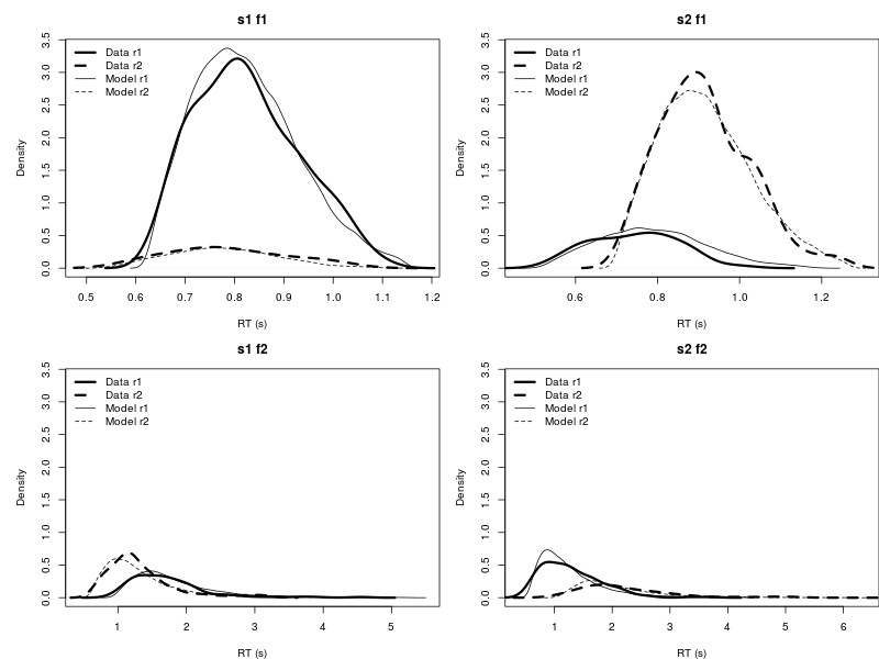
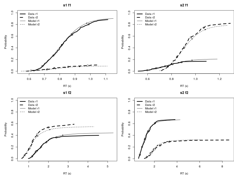
Posterior predictive check
You can also pipe the result to DMC to use its h.post.predict.dmc to conduct posterior predictive check at the hyper parameter. Note this will take a while, because piping back to DMC means using R language to process large Bayesian MCMC data. Further tutorials for DMC, please refer to Heathcote and colleagues (2018).
setwd("/media/yslin/MERLIN/Documents/DMCpaper/")
source ("dmc/dmc.R")
load_model ("LBA","lba_B.R")
setwd("/media/yslin/MERLIN/Documents/ggdmc_paper/")
hpp <- h.post.predict.dmc(hsam)
plot.pp.dmc(hpp)
tmp <- lapply(hpp, function(x){plot.pp.dmc(x, style = "cdf") })
Reference
Heathcote, A., Lin, Y.-S., Reynolds, A., Strickland, L., Gretton, M. & Matzke, D., (2018). Dynamic model of choice. Behavior Research Methods. https://doi.org/10.3758/s13428-018-1067-y.
-
a different way to store and manipulation data in R. ↩