This page (temporarily) documents four different plots for checking fitted models. The example simulates a data set from the regression normal model.

  rm(list = ls())
  model <- BuildModel(
    p.map     = list(a = "1", b = "1", tau = "1"),
    match.map = NULL,
    regressors= c(8, 15, 22, 29, 36),
    factors   = list(S = c("x1")),
    responses = "r1",
    constants = NULL,
    type      = "glm")
  p.vector <- c(a = 242.7, b = 6.185, tau = .01)
  ntrial <- 1000
  dat <- simulate(model, nsim = ntrial, ps = p.vector)
  dmi <- BuildDMI(dat, model)

  npar <- length(GetPNames(model))
  start <- BuildPrior(
    dists = c("tnorm2", "tnorm2", "gamma"),
    p1    = c(a = 240, b = 6, tau = .01),
    p2    = c(a = 1e-6, b = 1e-6, tau = .1),
    lower = c(NA, NA, NA),
    upper = rep(NA, npar))
  p.prior  <- BuildPrior(
    dists = c("tnorm2", "tnorm2", "gamma"),
    p1    = c(a = 200, b = 0, tau = .1),
    p2    = c(a = 1e-6, b = 1e-6, tau = .1),
    lower = c(NA, NA, NA),
    upper = rep(NA, npar))
  
  ## Sampling -----------
  fit0 <- Start_glm(5e2, dmi, start, p.prior, thin = 8)
  fit <- run(fit0, pm0 = .05)
  fit <- run(RestartSamples(5e2, fit, thin = 8))

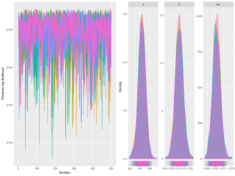
Trace and density plots

The first two are trace and density plots.

p0 <- plot(fit)
p1 <- plot(fit, pll = FALSE, den = TRUE)

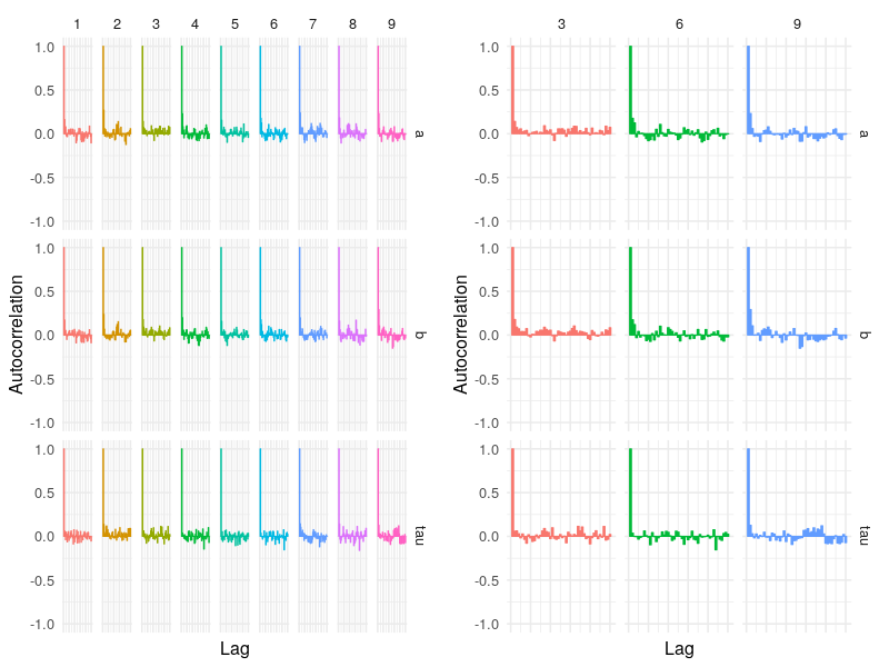
Autocorrelation plots

The third is the autocorrelation plot. This first figure plots all chains and the second randomly selects a subset of three chains to construct the figure. The latter function is useful when fitting a model with many parameters and the model fit uses a large number of chains. By default, the “autocor” calculates to 50 lags.

p2 <- autocor(fit)
p3 <- autocor(fit, nsubchain = 3)

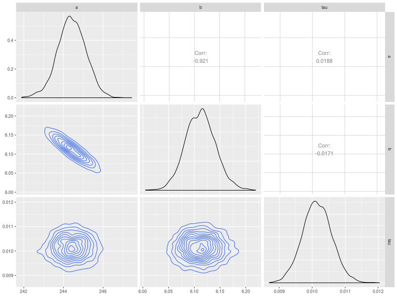
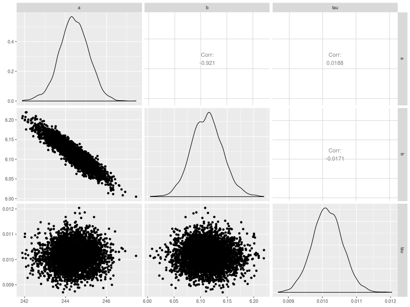
Correlation matrix

The fourth is the plot of correlation matrix. This plot is useful to check (post hoc) the association among model parameters. This needs to use the ggpairs function in GGally package.

pairs.model <- function(x, start = 1, end = NA, ...) {

  if (x$n.chains == 1) stop ("MCMC needs multiple chains to check convergence")
  if (is.null(x$theta)) stop("Use hyper mcmc_list")
  if (is.na(end)) end <- x$nmc
  if (end <= start) stop("End must be greater than start")

  d <- ConvertChains(x, start, end, FALSE)
  D_wide <- data.table::dcast.data.table(d, Iteration + Chain ~ Parameter, value.var = "value")

  bracket_names <- names(D_wide)
  par_cols <- !(bracket_names %in% c("Iteration", "Chain"))
  p0 <- GGally::ggpairs(D_wide, columnLabels = bracket_names[par_cols],
                        columns = which(par_cols), ...)
  print(p0)
  return(invisible(p0))
}

p5 <- pairs.model(fit)
p6 <- pairs.model(fit, lower = list(continuous = "density"))

The additional option in p6 is to choose to plot density contour.

lower = list(continuous = “density”)