Disclaimer: We have striven to minimize the number of errors. However, we cannot guarantee the note is 100% accurate. This tutorial requires the CDDM module, which is part of an ongoing research project, so has not released, yet.
Circular drift-diffusion model (CDDM) is a two-dimension process model. It could be viewed as an extension of the one-dimension diffusion model. One assumption of the 1-D diffusion model is it posits a single unit accumulator accrues evidence towards two opposing, an upper and a lower, boundaries. As illustrated in the right panel in the following figure, when the accumulator moves towards one boundary, it at the same time moves away from the other. This inevitable situation is in fact a powerful design that restricts the model to account for a set of processes. Therefore, the model provides a concise and successful account for the cognitive processes in the now ubiquitous two-alternative forced-choice (2AFC) task in cognitive psychology.
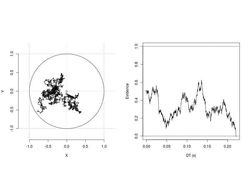 Figure 1. 1-D and 2-D random walk processes.
However, when one wants to model the tasks allowing more than two response types, it is not immediately clear how the 1-D diffusion model can extend to this situation. One usual option is to use the accumulator models (Ratcliff, Smith, Brown, & McKoon, 2016), for example, the LBA model, the LCA model or the feed forward inhibition model (Brown & Heathcote, 2008; Usher & McClellend, 2001; Mazurek et al., 2003; Niwa & Ditterich, 2008, Roe et al., 2001). These models use the absolute, as oppose to the relative, evidence criteria, as the stopping rule for the process. In this design, each response type corresponds to one unit accumulator, accuring evidence towards either one or multiple response thresholds.
Although it was discussed largely regarding to its utility to model the continuous report task (Smith, 2016), the circular drift-diffusion model can also account for the tasks with more than two responses. The aim of this tutorial is to demonstrate how this can be done using ggdmc. This tutorial is divided into three sections. First, we introduce three CDDM core functions, dcircle, rcircle, and rcircle_process. Following the convention of R language, d refers to probability density function and r refers to random number generation. Instead of recording only the response time and angle, rcircle_process simulates the 2-D diffusion process and records the trace, as shown in the left panel in the illustration figure. The source codes, CDDM.hpp and CDDM.cpp, provide the implementation details regarding the three functions.
In the second section, we replicated the simulation studies in Smith (2016) to check the accuracy of our CDDM module.
Next, we conducted a series of parameter recovery studies, using maximum likelihood estimation. The purpose of the recovery study is to provide a template when one wishes to fit an empirical data set from a continuous report task.
For using the Bayesian method to fit the CDDM, please go to the tutorials of fixed-effect and hierarchical models.
Core functions
The 2-D diffusion model has four main parameters, v1, v2, a, and t0. v1 and v2 are the average increments of the evidence on the x and y axes. They are the two components of the drift vector v, whose magnitude is the Euclidean norm ||v||.
\[\begin{align*} & || v || = \sqrt{v_1^2 + v_2^2} & \theta_v = tan^{-1}({v_2 / v1}) \end{align*}\]As the equation suggestes, a second way to describe the drift vector is via the left-hand side of the equation, using the magnitude and phase angle, \(\theta_v\) of the drift vector. The drift vector drives the evidence growth towards the decision boundary, a, which, in the case of 2-D diffusion model, is the circumference of a disc (Figure 1).
The stochastic component of the accumulation process is driven by the within-trial variability, \(\sigma^2\), the diffusion coefficient. For simplicity, the SD, \(\sigma\), corresponding to the two components of the drift vector are assumed as identical and independent of each other. We code it as sigma1 and sigma2 to remind the user that this is an assumption and the user can relax it by tweaking the source codes. For now, we recommend to set them as 1.
The time it takes the accumulator hit the boundary is the decision time. The response time is the decision time plus with the non-decision time, t0.
In summary, the parameter vector composes of:
- v1, the mean drift rate on the x axis,
- v2, the mean drift rate on the y axis,
- a, the response criterion,
- t0, the non-decision time
- sigma1, the within trial drift-rate standard deviation on the x axis,
- sigma2, the within trial drift-rate standard deviation on the y axis.
- eta1 and eta2 are two parameters related to the drift rate SD. They are usually set as 0.
Random-walk Process
Figure 1 was generated by the rcircle_process, the 2-D random-walk and r1d, the 1-D random-walk processes.
require(ggdmc)
## random walk 2d
## Set the upper bound of simulation time and each time step as 0.1 ms
tmax <- 2
h    <- 1e-4

p.vector <- c(v1=0, v2=0, a=1, t0=0, sigma1=1, sigma2=1, eta1=0, eta2=0)
res0 <- rcircle_process(P=p.vector, tmax=tmax, h=h)
str(res0)
## List of 3
##  $ out : num [1:3, 1] 0.732 -2.551 0
##  $ xPos: num [1:20001, 1] 0 0 0.0074 -0.0104 -0.0172 ...
##  $ yPos: num [1:20001, 1] 0 0 -0.0183 -0.0258 -0.0364 ...


## random walk 1d
p.vector <- c(v=0, a=1, z=.5, t0=0, s=1)
res1 <- r1d(P=p.vector, tmax=tmax, h=h)
idx <- sum(!is.na(res0$Xt)); idx
str(res1)
## List of 3
##  $ T  : num [1:20001, 1] 0e+00 1e-04 2e-04 3e-04 4e-04 5e-04 6e-04 7e-04 8e-04 9e-04 ...
##  $ out: num [1:2, 1] 0.221 0
##  $ Xt : num [1:20001, 1] 0.5 0.51 0.513 0.507 0.51 ...

## Plot the traces of 1-D and 2-D diffusion processes
png(filename='random_walk_2d.png', 800, 600)
par(mfrow=c(1,2), pty="s")
plotCircle(res0$xPos[,1], res0$yPos[,1], a=1)
plot(res1$T[1:idx], res1$Xt[1:idx], type='l', ylim=c(0, 1), xlab='DT (s)',
     ylab='Evidence')
abline(h=1, lty='dotted', lwd=1.5)
abline(h=0, lty='dotted', lwd=1.5)
points(x=0, y=p.vector[3], col='red')
dev.off()
Random number generation
To simulate multiple observations, rcircle allows the user to enter the number of observation via the n option. The implementation is simply a for loop running the code of the rcirle_process function repeatedly. Another useful option in rcircle is nw, which allows the user to divide the response angles into nw response categories.
n <- 150000
tmax <- 2
h <- 1e-4
p.vector <- c(v1=1, v2=1, a=1, t0=0, sigma1=1, sigma2=1, eta1=0, eta2=0)

## Took ~160 s. Divide the angles evenly into 11 categories
res0 <- rcircle(n=n, P=p.vector, tmax=tmax, h=h, nw=11)

d <- data.frame(res0)
names(d) <- c("R", "RT", "A")
## R stores the centered angles of the response category.
## A stores the actual hitting angles.
# dplyr::tbl_df(d)
# A tibble: 150,000 x 3
#         R    RT      A
#     <dbl> <dbl>  <dbl>
#  1 -0.286 0.116 -0.310
#  2  0.857 0.262  0.968
#  3 -0.286 0.329 -0.151
#  4  0.857 0.467  0.774
#  ...
# … with 149,990 more rows
Joint densities of zero-drift process
In the following, we simulated 50,000 observations from the zero-drift process by setting v1 and v2 to 0.
n <- 50000    ## 50,000 observations
h <- 1e-4     ## Define 0.1 ms as one time step
tmax <- 2     ## Define maximum decision time
nw <- 11      ## Divide the hitting angles into 11 categories
w <- 2*pi/nw  ## The width of each category of the hitting angles

## Define zero-drift parameter vector
p.vector <- c(v1=0, v2=0, a=1, t0=0, sigma1=1, sigma2=1, eta1=0, eta2=0)

## ~60 seconds
res0 <- rcircle(n=n, P=p.vector, tmax=tmax, h=h, nw=11)

## The simulation result is stored as a numerical matrix, so we convert it to
## an R data.frame
d <- data.frame(R = factor(round(res0[,1], 2)), RT = res0[,2], A = res0[,3])
Because we divide the hitting angles into 11 bins and are handeling bivariate data, we create a customerised histogram function to count the numbers of observation in each bin. Note one bin in this case is indexed by both the response times and hitting angles, so the densities, Gt, is a nw \(\times\) ntime matrix.
## See the end of this tutorial for the implementation of the function
res1 <- histogram_cddm(d, P=p.vector, nw=nw, tmax=tmax, h=h)

# List of 9
# $ Theta    : num [1:11] -3.142 -2.57 -1.999 -1.428 -0.857 ...
# $ Mt       : num [1:11] 0.499 0.514 0.51 0.5 0.511 ...
# $ Pt       : num [1:11] 0.161 0.158 0.156 0.158 0.163 ...
# $ time_grid: num [1:20001] 0e+00 1e-04 2e-04 3e-04 4e-04 5e-04 6e-04 7e-04 8e-04 9e-04 ...
# $ Gt       : num [1:11, 1:20001] 1.08e-16 9.96e-17 1.06e-16 9.77e-17 1.32e-16 ...
# $ Pmt      : num [1:11] 1 1 1 1 1 1 1 1 1 1 ...
# $ Mtscale  : num [1:11, 1:20001] 1 1 1 1 1 1 1 1 1 1 ...
# $ Gt_count : num [1:11, 1:20001] 0 0 0 0 0 0 0 0 0 0 ...
# $ d        :'data.frame':	220011 obs. of  3 variables:
#   ..$ R : Factor w/ 11 levels "-3.14","-2.57",..: 1 1 1 1 1 1 1 1 1 1 ...
#   ..$ RT: num [1:220011] 0e+00 1e-04 2e-04 3e-04 4e-04 5e-04 6e-04 7e-04 8e-04 9e-04 ...
#   ..$ D : num [1:220011] 1.90e-16 1.09e-16 2.21e-16 3.46e-17 2.05e-16 ...
Gt is the joint density matrix, with nw row and ntime column. The time grid is constructed based on the maximum simulation time, tmax and the user-defined time step, h. d is a data.frame, which rearranges the densities stored in Gt, the hitting angles stored in Theta, and the response times stored in time_grid.
Probability Density Function
dcircle calculates the predicted probability densities of the 2-D diffusion process.
den <- dcircle(d$RT, d$A, P=p.vector, tmax=tmax, kmax=50, sz=2/h, nw=50)
## Because den is a column vector. We convet it to a row vector.
d$D <- den[,1]
The following figure show the joing densities calculated from the simulations.
thetai <- levels(res1$d$R)

dat0 <- vector("list", length=nw)
dat1 <- vector("list", length=nw)
for(i in 1:nw) {
  tmp0 <- res1$d[res1$d$R==thetai[i],] ## simulation
  dat0[[i]] <- tmp0[order(tmp0$RT),]

  tmp1 <- d[d$R==thetai[i],]           ## predicted
  dat1[[i]] <- tmp1[order(tmp1$RT),]
}

colors <- RColorBrewer:::brewer.pal(9, "Set1")

par(pty='s')
plot(dat0[[1]]$RT, dat0[[1]]$D, col="grey60", ylim=c(0, .4),
     type='l', xlab='Time(s)', ylab='Joint density', cex.lab=2,
     cex.axis = 1.5)
lines(dat1[[1]]$RT, dat1[[1]]$D, lwd=2)

for(i in 2:nw)
{
  lines(dat0[[i]]$RT, dat0[[i]]$D, lwd=1, col=colors[i])
  lines(dat1[[i]]$RT, dat1[[i]]$D, lwd=2)
}
dev.off()
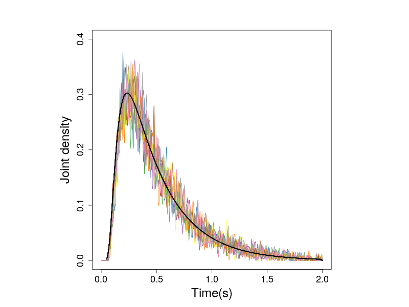 Figure 2. The joint densities of response times and response angles of zero-drift prcess. The black line shows the predicted densities.
Because the simulated observations are from the zero-drift process, the hitting angles do not affect the densities. This can be seen in Figure 3, which presents the histogrames in individual subplot.
## require ggplot2

x0 <- res1$d
x1 <- d
x0$TYPE <- 'Simulation'
x1$TYPE <- 'Prediction'
tmp0 <- x0[, c("RT", "D", "R", "TYPE")]
tmp1 <- x1[, c("RT", "D", "R", "TYPE")]
x2 <- rbind(tmp0, tmp1)

p0 <- ggplot(x2, aes(x=RT, y=D, colour=R)) +
  geom_line(aes(size=TYPE)) +
  scale_size_manual(values = c(1, .25) ) +
  xlab("RT(s)") + ylab("Joint density") +
  coord_cartesian(ylim=c(0, .4)) +
  facet_wrap(~R) +
  theme_bw(base_size=14) +
  theme(aspect.ratio=1,
        legend.position = 'none')

print(p0)
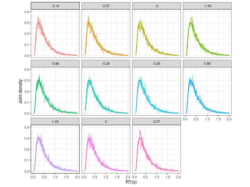 Figure 3. The upper panel shows the hitting-angle categories.
Similarly, we compare the predicted and simulated densities of the non-zero drift 2-D diffusion process.
## Test 1, nonzero-drift simulation --------
n <- 150000
tmax <- 2
h <- 1e-4
nw <- 11
p.vector <- c(v1=1, v2=1, a=1, t0=0, sigma1=1, sigma2=1, eta1=0, eta2=0)

## 179.4 s
res0 <- rcircle(n=n, P=p.vector, tmax=tmax, h=h, nw=nw)

d <- data.frame(R=factor(round(res0[,1], 2)), RT=res0[,2], A=res0[,3])
res1 <- histogram_cddm(d, P=p.vector, nw=nw, tmax=tmax, h=h)
x0 <- res1$d
thetai <- levels(res1$d$R)

## Predicted density -----------------------
res2 <- dcircle300(p.vector, tmax=2, kmax=50, sz=300, nw=nw)

x1  <- NULL
for(i in 1:nw) {
  x1 <- rbind(x1, data.frame(RT = res2$DT, A = rep(res2$R[i], 300), D = res2$Gt[i,]))
}

res3 <- divider(x1, nw=nw)
x1 <- dplyr::tbl_df(res3$d) ## overwrite x1

dplyr::tbl_df(x0)
dplyr::tbl_df(x1)

dat0 <- vector("list", length=nw)
dat1 <- vector("list", length=nw)
for(i in 1:nw) {
  tmp0 <- x0[x0$R==thetai[i],]
  dat0[[i]] <- tmp0[order(tmp0$RT),]

  tmp1 <- x1[x1$R==thetai[i],]
  dat1[[i]] <- tmp1[order(tmp1$RT),]
}


colors <- RColorBrewer:::brewer.pal(9, "Set1")

par(pty='s')
plot(dat0[[1]]$RT, dat0[[1]]$D, col="grey60", ylim=c(0, 1),
     type='l', xlab='Time(s)', ylab='Joint density', cex.lab=2,
     cex.axis = 1.5)
lines(dat1[[1]]$RT, dat1[[1]]$D)

for(i in 2:nw)
{
  lines(dat0[[i]]$RT, dat0[[i]]$D, lwd=1, col=colors[i])
  lines(dat1[[i]]$RT, dat1[[i]]$D, col=colors[i])
}

## ggplot 2
x0$TYPE <- 'Simulation'
x1$TYPE <- 'Prediction'
tmp0 <- x0[, c("RT", "D", "R", "TYPE")]
tmp1 <- x2[, c("RT", "D", "R", "TYPE")]
x2 <- rbind(tmp0, tmp1)

p0 <- ggplot(x2, aes(x=RT, y=D, colour=R)) +
  geom_line(aes(linetype = TYPE)) +
  xlab("DT(s)") + ylab("Joint density") +
  coord_cartesian(ylim=c(0, 1)) +
  # facet_wrap(~TYPE) +
  theme_bw(base_size=14) +
  theme(aspect.ratio=1,
        legend.position = 'none')
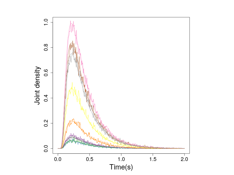 Figure 4. The nonzero probabiity densities of the 2-D diffusion process.
Helper functions
## This function is adpated from Smith's (2016) dirichlet1.m
histogram_cddm <- function(d, P, nw=11, tmax=2, h=1e-4)
{
  # d
  # pvec=p.vector
  # nw=11
  # tmax=2
  # h=1e-4
  v1 <- P[1];
  v2 <- P[2];
  a  <- P[3];
  t0 <- P[4]
  s1 <- P[5];
  s2 <- P[6];

  DT <- d[,2] - P[4]
  A  <- d[,3]

  ## Angles
  w <- 2*pi/nw
  Theta <- seq(-pi, pi-w, w)
  Thetabound <- c(Theta + w/2);

  ## Time
  time_grid <- seq(0, tmax, h)
  ntime_grid <- length(time_grid);
  tbound <- c(time_grid[1] - h/2, time_grid + h/2);

  Mt  <- Nt <- Pmt <- numeric(nw)
  Gt  <- Gt_count <- matrix(numeric(nw*ntime_grid), nrow=nw)

  n <- nrow(d)

  for (i in 1:n)
  {
    tmp0 <- which( A[i] <= Thetabound )
    thetaindex <- min( tmp0, na.rm=TRUE )

    ##  between -pi and Thetabound(1), pool into last
    if ( is.infinite(thetaindex) ) thetaindex <- 1

    tindex <- min( max( which( DT[i] > tbound) ), ntime_grid) ##  Pool into last bin.
    Nt[thetaindex] = Nt[thetaindex] + 1;
    Mt[thetaindex] = Mt[thetaindex] + DT[i];
    Gt[thetaindex,tindex]       <- Gt[thetaindex, tindex] + 1;
    Gt_count[thetaindex,tindex] <- Gt_count[thetaindex, tindex] + 1;
  }

  Mt <- Mt / Nt; ## Average time per theta group
  Pt <- Nt / n;

  ## Gt densities
  filter <- cos( seq(-pi/2, pi/2, .025))
  filter <- filter / sum(filter);  #  Normalize mass in filter

  for (i in 1:nw)
  {
    Gtfi <- pracma::conv(Gt[i,], filter)
    ## %Gt(i,:) = Gtfi(1:szt)./(Nt(i) * h +eps); % conditional
    Gt[i,] <- Gtfi[1:ntime_grid] / (n  * h);  ## % joint density
  }

  for (i in 1:nw) {
    Pmt[i] <- exp(a*cos(Theta[i])*v1 / s1^2 + a*sin(Theta[i])*v2 / s2^2)
  }

  Commonscale <-  exp(-0.5 * (v1^2/s1^2 + v2^2/s2^2) * time_grid);
  # Multiply theta-dependent drift term by invariant time-dependent term
  Mtscale <- as.matrix(Pmt) %*% Commonscale;
  Pt <- Pt / w; # % To make into a density estimate.


  thidx <- factor(round(Theta, 2))
  ## ------------------------------------------------------------------------##
  ## Note that to get the joint density of hitting
  ## angles and resposne times, the densities were divided by w
  ## ------------------------------------------------------------------------##
  x0 <- NULL
  for(i in 1:nw) {
    tmp0 <- data.frame(R = thidx[i], RT = time_grid+t0, D = Gt[i,]/w)
    x0 <- rbind(x0, tmp0)
  }


  return(list(Theta=Theta, Mt=Mt, Pt=Pt, time_grid=time_grid, Gt=Gt, Pmt=Pmt,
              Mtscale=Mtscale, Gt_count=Gt_count, d=x0))
}