- We have striven to minimize the number of errors. However, we canot guarantee the note is 100% accurate.
- We have updated the predict_one function for S4 class (19/01/2020).
- This update is tested on Ubuntu 18.04.3 LTS (Intel® Core™ i5-8400 CPU @ 2.80GHz × 6; Memory: 7.7 GB)
This is a quick note for fitting 3-accumulator LBA model. First, some pre-analysis set up work.
## version 0.2.7.8
## devtools::install_github("yxlin/ggdmc")
loadedPackages <-c("ggdmc", "data.table", "ggplot2", "gridExtra", "ggthemes")
sapply(loadedPackages, require, character.only=TRUE)

## A function for generating posterior predictive samples for one participant fit
predict_one <- function(object, npost = 100, xlim = NA, seed = NULL)
{
    facs   <- attr(object@dmi@model, "factors");
    fnames <- names(facs);
    ns <- table( object@dmi@data[, fnames], dnn = fnames)
    nsample <- object@nchain * object@nmc;
    pnames <- object@pnames;

    thetas <- matrix(aperm(object@theta, c(3,2,1)), ncol = object@npar)
    colnames(thetas) <- pnames

    if (is.na(npost)) stop("Must specify npost!")

    use    <- sample(1:nsample, npost, replace = FALSE);
    npost  <- length(use)
    posts  <- thetas[use, ]
    ntrial <- sum(ns)
    v <- lapply(1:npost, function(i) {
        simulate(object@dmi@model, nsim = ns, ps = posts[i,], seed = seed)
    })
    out <- data.table::rbindlist(v)
    reps <- rep(1:npost, each = ntrial)
    out <- cbind(reps, out)

    if (!any(is.na(xlim))) out <- out[RT > xlim[1] & RT < xlim[2]]
    attr(out, "data") <- object@dmi
    return(out)
}
In this example, we assumed three accumulators corresponding to three responses. Let’s say they are “Word”, “Nonword”, and “Pseudo-word”. They are coded respectively as W, N and P. This is to assume we had run some (visual) lexical-decision experiments, instructing participants to decide whether a stimulus is a word, a non-word, or a make-up word. The three types of stimuli are coded as ww, nn and pn.
model <- BuildModel(
  p.map     = list(A = "1", B = "1", t0 = "1", mean_v = "R", sd_v = "1",
                   st0 = "1"),
  match.map = list(M = list(ww = "W", nn = "N", pn = "P")),
  factors   = list(S = c("ww", "nn", "pn")),
  constants = c(st0 = 0, sd_v = 1),
  responses = c("W", "N", "P"),
  type      = "norm")
## Parameter vector names are: ( see attr(,"p.vector") )
## [1] "A"        "B"        "t0"       "mean_v.W" "mean_v.N" "mean_v.P"
##
## Constants are (see attr(,"constants") ):
##  st0 sd_v
##    0    1
##
## Model type = norm (posdrift = TRUE )
Firstly, as usual, we conducted a small recovery study. That is, we designated a parameter vector with specific values and on the basis of this particular parameter vector, we simulated a data set and fit such data set with the model to see if it could recover the values reasonably well.
For now, we will show only the recovery study.
p.vector <- c(A = 1.25, B = .25, t0 = .2, mean_v.W = 2.5, mean_v.N = 1.5,
              mean_v.P = 1.2)

## ggdmc adapts print function to help inspect model
print(model)

## The model array is huge
## W
##         A    B   t0 mean_v.W mean_v.N mean_v.P sd_v  st0
## ww.W TRUE TRUE TRUE     TRUE    FALSE    FALSE TRUE TRUE
## nn.W TRUE TRUE TRUE     TRUE    FALSE    FALSE TRUE TRUE
## pn.W TRUE TRUE TRUE     TRUE    FALSE    FALSE TRUE TRUE
## ww.N TRUE TRUE TRUE     TRUE    FALSE    FALSE TRUE TRUE
## nn.N TRUE TRUE TRUE     TRUE    FALSE    FALSE TRUE TRUE
## pn.N TRUE TRUE TRUE     TRUE    FALSE    FALSE TRUE TRUE
## ww.P TRUE TRUE TRUE     TRUE    FALSE    FALSE TRUE TRUE
## nn.P TRUE TRUE TRUE     TRUE    FALSE    FALSE TRUE TRUE
## pn.P TRUE TRUE TRUE     TRUE    FALSE    FALSE TRUE TRUE
## N
##         A    B   t0 mean_v.W mean_v.N mean_v.P sd_v  st0
## ww.W TRUE TRUE TRUE    FALSE     TRUE    FALSE TRUE TRUE
## nn.W TRUE TRUE TRUE    FALSE     TRUE    FALSE TRUE TRUE
## pn.W TRUE TRUE TRUE    FALSE     TRUE    FALSE TRUE TRUE
## ww.N TRUE TRUE TRUE    FALSE     TRUE    FALSE TRUE TRUE
## nn.N TRUE TRUE TRUE    FALSE     TRUE    FALSE TRUE TRUE
## pn.N TRUE TRUE TRUE    FALSE     TRUE    FALSE TRUE TRUE
## ww.P TRUE TRUE TRUE    FALSE     TRUE    FALSE TRUE TRUE
## nn.P TRUE TRUE TRUE    FALSE     TRUE    FALSE TRUE TRUE
## pn.P TRUE TRUE TRUE    FALSE     TRUE    FALSE TRUE TRUE
## P
##         A    B   t0 mean_v.W mean_v.N mean_v.P sd_v  st0
## ww.W TRUE TRUE TRUE    FALSE    FALSE     TRUE TRUE TRUE
## nn.W TRUE TRUE TRUE    FALSE    FALSE     TRUE TRUE TRUE
## pn.W TRUE TRUE TRUE    FALSE    FALSE     TRUE TRUE TRUE
## ww.N TRUE TRUE TRUE    FALSE    FALSE     TRUE TRUE TRUE
## nn.N TRUE TRUE TRUE    FALSE    FALSE     TRUE TRUE TRUE
## pn.N TRUE TRUE TRUE    FALSE    FALSE     TRUE TRUE TRUE
## ww.P TRUE TRUE TRUE    FALSE    FALSE     TRUE TRUE TRUE
## nn.P TRUE TRUE TRUE    FALSE    FALSE     TRUE TRUE TRUE
## pn.P TRUE TRUE TRUE    FALSE    FALSE     TRUE TRUE TRUE
## The model object carries this many attributes
## Attributes:
##  [1] "dim"        "dimnames"   "all.par"    "p.vector"   "par.names"  "type"       "factors"
##  [8] "responses"  "constants"  "posdrift"   "n1.order"   "match.cell" "match.map"  "is.r1"
## [15] "class"


print(model, p.vector)
## The following is how ggdmc allocates the parameters to each accumulator.
## [1] "ww.W"
##      A   b  t0 mean_v sd_v st0
## 1 1.25 1.5 0.2    2.5    1   0
## 2 1.25 1.5 0.2    1.5    1   0
## 3 1.25 1.5 0.2    1.2    1   0
## [1] "nn.W"
##      A   b  t0 mean_v sd_v st0
## 1 1.25 1.5 0.2    2.5    1   0
## 2 1.25 1.5 0.2    1.5    1   0
## 3 1.25 1.5 0.2    1.2    1   0
## [1] "pn.W"
##      A   b  t0 mean_v sd_v st0
## 1 1.25 1.5 0.2    2.5    1   0
## 2 1.25 1.5 0.2    1.5    1   0
## 3 1.25 1.5 0.2    1.2    1   0
...

## To see what other options in the simulate function
## ?ggdmc:::simulate
nsim <- 2048
dat <- simulate(model, nsim = nsim, ps = p.vector)
We used data.table to inspect the data frame. This makes no difference when the data set is small.
d <- data.table(dat)
dmi <- BuildDMI(dat, model)

## Check the factor levels
sapply(d[, .(S,R)], levels)
##     S    R
## [1,] "ww" "W"
## [2,] "nn" "N"
## [3,] "pn" "P"
To inspect the response time distributions, we designated the response proportions for each of the response types.
ww1 <- d[S == "ww" & R == "W" & RT <= 10, "RT"]
ww1 <- d[S == "ww" & R == "W" & RT <= 10, "RT"]
ww2 <- d[S == "ww" & R == "N" & RT <= 10, "RT"]
ww3 <- d[S == "ww" & R == "P" & RT <= 10, "RT"]
nn1 <- d[S == "nn" & R == "W" & RT <= 10, "RT"]
nn2 <- d[S == "nn" & R == "N" & RT <= 10, "RT"]
nn3 <- d[S == "nn" & R == "P" & RT <= 10, "RT"]
pn1 <- d[S == "pn" & R == "W" & RT <= 10, "RT"]
pn2 <- d[S == "pn" & R == "N" & RT <= 10, "RT"]
pn3 <- d[S == "pn" & R == "P" & RT <= 10, "RT"]

xlim <- c(0, 5)
par(mfrow=c(1, 3), mar = c(4, 4, 0.82, 1))
hist(ww1$RT, breaks = "fd", freq = TRUE, xlim = xlim, main='Word', xlab='RT(s)',
     cex.lab=1.5)
hist(ww2$RT, breaks = "fd", freq = TRUE, add = TRUE, col = "lightblue")
hist(ww3$RT, breaks = "fd", freq = TRUE, add = TRUE, col = "orange")

hist(nn1$RT, breaks = "fd", freq = TRUE, xlim = xlim, main='Non-word',
     xlab='RT(s)', ylab='', cex.lab=1.5)
hist(nn2$RT, breaks = "fd", freq = TRUE, add = TRUE, col = "lightblue")
hist(nn3$RT, breaks = "fd", freq = TRUE, add = TRUE, col = "orange")

hist(pn1$RT, breaks = "fd", freq = TRUE, xlim = xlim, main='Pseudo-word',
     xlab='RT(s)', ylab='', cex.lab=1.5)
hist(pn2$RT, breaks = "fd", freq = TRUE, add = TRUE, col = "lightblue")
hist(pn3$RT, breaks = "fd", freq = TRUE, add = TRUE, col = "orange")
par(mfrow=c(1, 1))
Prior distribution
p.prior <- BuildPrior(
  dists = c("tnorm", "tnorm", "beta", "tnorm", "tnorm", "tnorm"),
  p1    = c(A = .3, B = 1, t0 = 1,
            mean_v.W = 1, mean_v.N = 0, mean_v.P = .1),
  p2    = c(1, 1,   1,  3, 3, 3),
  lower = c(0, 0,   0, NA, NA, NA),
  upper = c(NA, NA, 1, NA, NA, NA))

## Visually check the prior distributions
plot(p.prior, ps = p.vector)
Sampling
The default number of iteration is 200 for StartNewsamples function.
## ?run to see add and other options in run function
fit0 <- StartNewsamples(dmi, p.prior, thin = 2)
fit <- run(fit0, thin = 2, block = FALSE)
## gelman function also provide subchain option.
## Note the method to call this option is different
res <- gelman(fit, verbose = TRUE, subchain = 1:3)
## Calculate chains: 1 2 3
## Multivariate psrf:
## Point est. Upper C.I.
## A 1.02 1.08
## B 1.00 1.01
## t0 1.01 1.01
## mean_v.W 1.01 1.03
## mean_v.N 1.01 1.03
## mean_v.P 1.01 1.02
## By convention, most Bayesian inference checks 3 or 4 chains
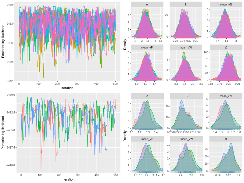
p1 <- plot(fit)
p2 <- plot(fit, pll=F, den=T)
p3 <- plot(fit, subchain = TRUE)
p4 <- plot(fit, pll=F, den=T, subchain = TRUE)
png(file = "LBA3A-checks.png", 800, 600)
grid.arrange(p1, p2, p3, p4)
dev.off()
es <- effectiveSize(fit, verbose = TRUE)
##        A        B       t0 mean_v.W mean_v.N mean_v.P
##   843.04   838.92   863.98   828.97   840.93   894.25

est <- summary(fit, ps = p.vector, verbose = TRUE, recovery = TRUE)
## Recovery summarises only default quantiles: 2.5% 25% 50% 75% 97.5%
##                     A       B mean_v.N mean_v.P mean_v.W     t0
## True           1.2500  0.2500   1.5000   1.2000   2.5000 0.2000
## 2.5% Estimate  1.1516  0.2153   1.3745   1.0190   2.3058 0.1900
## 50% Estimate   1.2724  0.2495   1.5667   1.2116   2.5075 0.2000
## 97.5% Estimate 1.4053  0.2920   1.7573   1.4070   2.7250 0.2085
## Median-True    0.0224 -0.0005   0.0667   0.0116   0.0075 0.0000
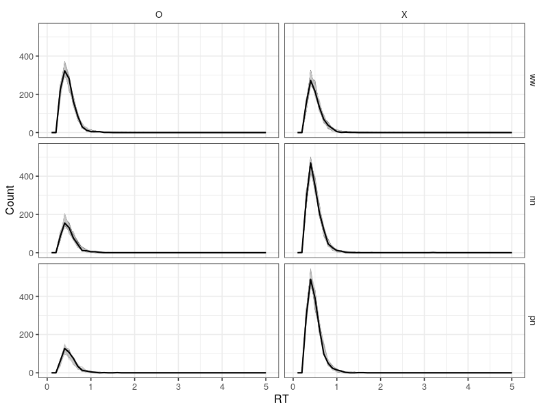
The posterior predictive figure shows the data and posterior predictions are consistent, confirming the model does work well.
pp <- predict_one(fit, xlim = c(0, 5))

original_data <- fit@dmi@data
dplyr::tbl_df(original_data)
d <- data.table(original_data)

## A different way to check data frame
dplyr::tbl_df(original_data)
d <- data.table(original_data)

## Response proportions
d[, .N, .(S)]
d[, .N/100, .(S, R)]


## Score for the correct and error response
dat$C <- ifelse(dat$S == "ww" & dat$R == "W", "O",
         ifelse(dat$S == "nn" & dat$R == "N", "O",
         ifelse(dat$S == "pn" & dat$R == "P", "O",
         ifelse(dat$S == "ww" & dat$R == "N", "X",
         ifelse(dat$S == "ww" & dat$R == "P", "X",
         ifelse(dat$S == "nn" & dat$R == "W", "X",
         ifelse(dat$S == "nn" & dat$R == "P", "X",
         ifelse(dat$S == "pn" & dat$R == "N", "X",
         ifelse(dat$S == "pn" & dat$R == "W", "X", NA)))))))))

pp$C <- ifelse(pp$S == "ww" & pp$R == "W", "O",
        ifelse(pp$S == "nn" & pp$R == "N", "O",
        ifelse(pp$S == "pn" & pp$R == "P", "O",
        ifelse(pp$S == "ww" & pp$R == "N", "X",
        ifelse(pp$S == "ww" & pp$R == "P", "X",
        ifelse(pp$S == "nn" & pp$R == "W", "X",
        ifelse(pp$S == "nn" & pp$R == "P", "X",
        ifelse(pp$S == "pn" & pp$R == "N", "X",
        ifelse(pp$S == "pn" & pp$R == "W", "X", NA)))))))))


dat0 <- dat
dat0$reps <- NA
dat0$type <- "Data"
pp$reps <- factor(pp$reps)
pp$type <- "Simulation"
combined_data <- rbind(dat0, pp)

dplyr::tbl_df(combined_data)

p1 <- ggplot(combined_data, aes(RT, color = reps, size = type)) +
  geom_freqpoly(binwidth = .10) +
  scale_size_manual(values = c(1, .3)) +
  scale_color_grey(na.value = "black") +
  ylab("Count") +
  facet_grid(S ~ C) +
  theme_bw(base_size = 16) +
  theme(strip.background = element_blank(),
        legend.position="none")

png(file = "LBA3A.png", 800, 600)
print(p1)
dev.off()
Extending to four or more accumulators
Here is a barebone template of 4 stimuli mapping to 4 responses. This is a 15-parameter model; thus, one should expect it would take up a lot of computation time, especially in fitting hierarchical model. It would save time, if one fits fixed-effect model first, using multiple cores.
require(ggdmc)
## Assume four stimuli that have a shape and color (blue_diamond, blue_heart,
## green_diamond, and green_heart) (courtesy of davidt0x)
##
## I assume a difficulty hierarchy (with no theoretical basis) (from easy to hard): green_diamond (e1) > green_heart (e2) > blue_diamond (e3) > blue_heart (e4). I also assume the easier stimulus, the higher its drift rate is and the more variable (hence the higher value) its drift rate standard deviation would be.

model <- BuildModel(
    p.map     = list(A = "1", B = "R", t0 = "1", mean_v = c("S", "M"),
                     sd_v = "M", st0 = "1"),
    match.map = list(M = list("blue_diamond" = "BD", "blue_heart" = "BH",
                              "green_diamond" = "GD", "green_heart" = "GH")),
    factors   = list(S = c("blue_diamond", "blue_heart", "green_diamond", "green_heart")),
    constants = c(sd_v.false = 1, st0 = 0),
    responses = c("BD", "BH", "GD", "GH"),
    type      = "norm")

pop.mean <- c(A=.4, B.BD=.5, B.BH=.6, B.GD=.7, B.GH=.8,
              t0=.3,
              mean_v.blue_diamond.true   = 1.5,
              mean_v.blue_heart.true     = 1.0,
              mean_v.green_diamond.true  = 2.5,
              mean_v.green_heart.true    = 2.0,
              mean_v.blue_diamond.false  = .20,
              mean_v.blue_heart.false    = .25,
              mean_v.green_diamond.false = .10,
              mean_v.green_heart.false   = .15,
              sd_v.true = .25)

pop.scale <-c(A=.1, B.BD=.1, B.BH=.1, B.GD=.1, B.GH=.1,
              t0=.05,
              mean_v.blue_diamond.true   = .2,
              mean_v.blue_heart.true     = .2,
              mean_v.green_diamond.true  = .2,
              mean_v.green_heart.true    = .2,
              mean_v.blue_diamond.false  = .2,
              mean_v.blue_heart.false    = .2,
              mean_v.green_diamond.false = .2,
              mean_v.green_heart.false   = .2,
              sd_v.true = .1)

pop.prior <- BuildPrior(
     dists = rep("tnorm", model@npar),
     p1 = pop.mean,
     p2 = pop.scale,
     lower = c(0,0,0,0,0,        .05, NA,NA,NA,NA, NA,NA,NA,NA, 0),
    upper = c(NA,NA,NA,NA,NA,    1, NA,NA,NA,NA, NA,NA,NA,NA, NA))

## plot(pop.prior)
## Simulate some data ----------
## Assume 12 participants, each contributing 30 trials per condition.
dat <- simulate(model, nsub = 12, nsim = 30, prior = pop.prior)
dmi <- BuildDMI(dat, model)
ps <- attr(dat, "parameters")

p.prior <- BuildPrior(
    dists = rep("tnorm", model@npar),
    p1   = pop.mean,
    p2   = pop.scale*5,
    lower = c(0,0,0,0,0,        .05, NA,NA,NA,NA, NA,NA,NA,NA, 0),
    upper = c(NA,NA,NA,NA,NA,    1, NA,NA,NA,NA, NA,NA,NA,NA, NA))

mu.prior <- BuildPrior(
    dists = rep("tnorm",  model@npar),
    p1    = pop.mean,
    p2    = c(1,1,1,1,1,  1, 2,2,2,2, 2,2,2,2, 2),
    lower = c(0,0,0,0,0,       .05, NA,NA,NA,NA, NA,NA,NA,NA, 0),
    upper = c(NA,NA,NA,NA,NA,    1, NA,NA,NA,NA, NA,NA,NA,NA, NA))

plot(p.prior, ps=ps)
plot(mu.prior, ps = pop.mean)

sigma.prior <- BuildPrior(
    dists = rep("unif", model@npar),
    p1    = c(A = 0, B.BD = 0, B.BH = 0, B.GD=0, B.GH=0,
              t0 = 0,
              mean_v.blue_diamond.true   = 0,
              mean_v.blue_heart.true     = 0,
              mean_v.green_diamond.true  = 0,
              mean_v.green_heart.true    = 0,
              mean_v.blue_diamond.false  = 0,
              mean_v.blue_heart.false    = 0,
              mean_v.green_diamond.false = 0,
              mean_v.green_heart.false   = 0,
              sd_v.true = 0),
    p2    = rep(5, model@npar))

## plot(sigma.prior, ps=pop.scale)
## Sampling -------------
priors <- list(pprior=p.prior, location=mu.prior, scale=sigma.prior)

## Enter only the participant-level prior distribution will render the function to
## run fixed-effect model
## Use nmc = 10 to estimate how much time would take.
## 42.22

fit0 <- StartNewsamples(dmi, prior=p.prior, block = FALSE, ncore=12)  ## Fixed-effect model fit
fit  <- run(fit0, ncore = 12, block = FALSE)

hfit0 <- StartNewsamples(dmi, prior=priors)  ## Random-effect model fit
hfit  <- run(hfit0)      ## ncore has no effect in hierarchical fit


## Model diagnoses
plot(fit)
plot(fit, subchain=TRUE, nsubchain=3)
plot(fit, subchain=TRUE, nsubchain=2)

res <- gelman(fit, verbose = TRUE)
res <- gelman(fit, verbose = TRUE, subchain=1:4)
res <- gelman(fit, verbose = TRUE, subchain=5:8)
res <- gelman(fit, verbose = TRUE, subchain=9:12)

## Check if parameter recovery well in fixed-effect model fit
est0 <- summary(fit, recovery = TRUE, ps = ps, verbose =TRUE)
How to fix array dimension inconsistency
If data were stored by a previous version of ggdmc or by DMC, their arraies are arranged differently as noted here. The following is one convenient way to transpose them.
## First make sure they are indeed needed to be transposed
dim(fit0@theta)
dim(fit0@summed_log_prior)
dim(fit0@log_likelihoods)

dim(fit0$theta)
dim(fit0$summed_log_prior)
dim(fit0$log_likelihoods)

## Use aperm and t to transpose arrays and matrices
fit0@theta <- aperm(fit0@theta, c(2, 1, 3))
fit0@summed_log_prior <- t(fit0@summed_log_prior)
fit0@log_likelihoods <- t(fit0@log_likelihoods)

## Make the new object a posterior class
class(fit0) <- c("posterior")