I continued the shooting decision model by fitting the empirical data in study 1 in Pleskac, Cesario and Johnson (2017). First I started from the pre-processing of the data. The aim of the pre-process is to replicate their behaviour analysis, so I can be sure that my data pre-processing is in line with theirs.
First, I used a combination of sapply and table functions to check all coding numbers in the categorical variables / columns.
require(ggdmc)
dat <- fread("data/race/Study1TrialData.csv")
dplyr::tbl_df(dat)
##  A tibble: 5,600 x 11
##    subject race0W1B object0NG1G conditionRaceObj conditionRace    rt resp0DS1S
##      <int>    <int>       <int>            <int>         <int> <dbl>     <dbl>
##  1       1        1           1                4             2   464         1
##  2       1        1           0                2             2   658         0
##  3       1        1           1                4             2   776         1
##  4       1        0           1                3             1   646         1
##  5       1        0           0                1             1   624         0
##  6       1        0           1                3             1   518         1
##  7       1        1           0                2             2   678         0
##  8       1        0           1                3             1   511         1
##  9       1        0           0                1             1   602         1
## 10       1        1           1                4             2   808         1
##  ... with 5,590 more rows, and 4 more variables: diffusionRT <dbl>, ybin <int>,
##    lowerLim <dbl>, upperLim <dbl>

sapply(dat[, c("subject", "race0W1B", "object0NG1G", "conditionRaceObj",
               "conditionRace", "resp0DS1S")], table)
## $subject
##
##   1   2   3   4   5   6   7   8   9  10  11  12  13  14  15  16  17  18  19  20  21  22
## 100 100 100 100 100 100 100 100 100 100 100 100 100 100 100 100 100 100 100 100 100 100
##  23  24  25  26  27  28  29  30  31  32  33  34  35  36  37  38  39  40  41  42  43  44
## 100 100 100 100 100 100 100 100 100 100 100 100 100 100 100 100 100 100 100 100 100 100
##  45  46  47  48  49  50  51  52  53  54  55  56
## 100 100 100 100 100 100 100 100 100 100 100 100
##
## $race0W1B
##
##    0    1
## 2800 2800
##
## $object0NG1G
##
##    0    1
## 2800 2800
##
## $conditionRaceObj
##
##    1    2    3    4
## 1400 1400 1400 1400
##
## $conditionRace
##
##    1    2
## 2800 2800
##
## $resp0DS1S
##
##    0    1
## 2636 2796
Second, I relabeled their numerical coding to character strings, using ifelse and factor functions. In the “object0NG1G” for example, ifelse function finds “0” and converts it to “non”, meaning non-gun condition. Otherwise, it converts any numbers it found to “gun”, meaning gun condition. Because I have used table to check all available numbers, leaving all other number to else is OK. factor function converts the integer column (which will be interpreted as continuous variable) to categorical (i.e., nominal) variables.
Next, I used the data.table way to remove the redundant columns, because I have reformatted them to follow our convention / standard (e.g., using single uppercase letters referring to experimental factors).
dat$S    <- factor(ifelse(dat$object0NG1G == 0, "non", "gun"))
dat$RACE <- factor(ifelse(dat$race0W1B == 0, "white", "black"))
dat$R    <- factor(ifelse(dat$resp0DS1S == 0, "not", "shoot"))
dat$RT   <- dat$rt / 1e3
dat$s    <- factor(dat$subject)
dat[, c("subject", "race0W1B", "object0NG1G", "conditionRaceObj",
  "conditionRace", "rt", "resp0DS1S", "diffusionRT", "ybin", "lowerLim", "upperLim") := NULL]
Real data sets often contain some abnormal responses, such as outliers, very slow, very quick, and wrong key responses. I used is.nan function to check whether the RT columns have this type of responses. is.nan returns a logical vector, indicating that if an element it found is “Not a number”, it will return FALSE, otherwise TRUE. I then added all elements in the vector to see how many TRUEs (1) are there. Logical TRUE in R is interpreted as 1, relative to logical FALSE, which is interpreted as 0.
I found there are 168 such responses, which I removed them by a simple data.table syntax and stored the result as d.
is.nan(dat$RT)
## FALSE FALSE FALSE FALSE FALSE FALSE ...
sum(is.nan(dat$RT))
## [1] 168
d <- dat[!is.nan(dat$RT)]
To help the calculation of the proportions of correct and error responses, I created two logical columns, C and error, to store whether a trial records a correct or error response.
d$C <- ifelse(d$S == "gun"  & d$R == "shoot",  TRUE,
       ifelse(d$S == "non" & d$R == "not", TRUE,
       ifelse(d$S == "gun"  & d$R == "not", FALSE,
       ifelse(d$S == "non" & d$R == "shoot",  FALSE, NA))))
d$error <- ifelse(d$S == "gun"  & d$R == "shoot",  FALSE,
           ifelse(d$S == "non" & d$R == "not", FALSE,
           ifelse(d$S == "gun"  & d$R == "not", TRUE,
           ifelse(d$S == "non" & d$R == "shoot",  TRUE, NA))))
Next I examine how many trials in each experimental condition. This can be achieved by a simple data.table syntax.
d[, .N, .(s, S,  RACE)]
#        s    S  RACE  N
#   1:   1  gun black 25
#   2:   1  non black 25
#   3:   1  gun white 25
#   4:   1  non white 25
#   5:   2  non black 25
# ---
# 220:  55  non white 25
# 221:  56  gun black 25
# 222:  56  gun white 25
# 223:  56  non black 25
# 224:  56  non white 25
Applying table function on the N column in the above resulting data table, I can check exactly the per-condition trial numbers.
table(d[, .N, .(s, S, RACE)]$N)
## 19  21  22  23  24  25
##  1   3  11  33  51 125
There are six trial numbers: 19, 21, 22, 23, 24, 25, with mostly subject-conditions combination (125) have 25 trials.
nrow(d[, .N, .(s)])
unique(d$s)
## Fig. 3
source("~/rc/data.analysis.R")
source("~/rc/utils.R")
source("~/functions/summarise.R")
d
acc0 <- summarySE(d, mv = "error", gvs = c("s", "RACE", "S"))
mrt0 <- summarySE(d[C == TRUE], mv = "RT",    gvs = c("s", "RACE", "S"))
## Within se average across subjects for pc and nt
figA <- summarySEwithin(acc0, wvs = c("RACE", "S"), mv = "error")
figB <- summarySEwithin(mrt0, wvs = c("RACE", "S"), mv = "RT")
names(figA) <- c("RACE", "S", "N", "y", "sd", "se", "ci")
names(figB) <- c("RACE", "S", "N", "y", "sd", "se", "ci")
head(figA)
dplyr::tbl_df(figA)
levels(figA$RACE)
figA$RACE <- factor(figA$RACE, levels = c("white", "black"), labels = c("White", "Black"))
figA$S <- factor(figA$S, levels = c("non", "gun"), labels = c("Non-Gun", "Gun"))
# figA$gp   <- factor(paste(figA$CT, figA$S),
#   levels = c("safe non", "safe gun", "danger non", "danger gun"),
#   labels = c("Neutral Non-Gun", "Neutral Gun", "Dangerous Non-Gun", "Dangerous Gun"))

figB$RACE <- factor(figB$RACE, levels = c("white", "black"), labels = c("White", "Black"))
figB$S <- factor(figB$S, levels = c("non", "gun"), labels = c("Non-Gun", "Gun"))
# figB$gp   <- factor(paste(figB$CT, figB$S),
#   levels = c("safe non", "safe gun", "danger non", "danger gun"),
#   labels = c("Neutral Non-Gun", "Neutral Gun", "Dangerous Non-Gun", "Dangerous Gun"))

# figA$parameter <- "ER"
# figB$parameter <- "RT"
# fig7 <- rbind(figA, figB)
# head(fig7)
# Error bars represent standard error of the mean
p1 <- ggplot(figA, aes(x = S, y = y, fill = RACE)) +
  geom_bar(position = position_dodge(), color = "black", stat="identity") +
  geom_errorbar(aes(ymin = y - se, ymax = y + se), width=.1,
    position=position_dodge(.9)) +
  coord_cartesian(ylim = c(0, .20)) +
  scale_fill_manual(values = c("#FFFFFF", "#CCCCCC")) +
  ylab("Error Rate") +
  coord_cartesian(ylim = c(0, .08)) +

  # facet_grid(.~BC) +
  theme_bw() +
  theme(legend.position = c(.85, .75),
    strip.background = element_blank(),
    axis.title.y = element_text(size = 20),
    strip.text.x = element_text(size = 18),
    axis.title.x = element_blank(),
    axis.ticks.x = element_blank(),
    axis.text.y = element_text(size = 18),
    axis.text.x = element_blank())

p2 <- ggplot(figB, aes(x = S, y = y, fill = RACE)) +
  geom_bar(position = position_dodge(), color = "black", stat="identity") +
  geom_errorbar(aes(ymin = y - se, ymax = y + se), width=.1,
    position=position_dodge(.9)) +
  scale_fill_manual(values = c("#FFFFFF", "#CCCCCC")) +
  ylab("Correct Response Time (s)") +
  coord_cartesian(ylim = c(.54, .65)) +
  # facet_grid(.~BC) +
  theme_bw() +
  theme(legend.position = "none",
    strip.text.x = element_blank(),
    axis.title.y = element_text(size = 20),
    axis.text.x = element_text(size = 18),
    axis.text.y = element_text(size = 18),
    axis.title.x = element_blank())


png("figs/race/fig3.png", 800, 600)
grid.arrange(p1, p2, ncol = 1)
dev.off()

save(dat, d, file = "data/race/study1.rda")


load("data/race/study1.rda")

load("data/race/shoot-decision-recovery.rda")

study3_subset <- study3[, c("s", "S", "RACE", "R", "RT")]
dplyr::tbl_df(study3_subset)

## A tibble: 12,033 x 5
##     s     S     RACE   R     RT
##    <fct> <fct> <fct> <fct> <dbl>
##  1 11    gun   black not   0.753
##  2 11    non   white shoot 0.851
##  3 11    gun   black not   0.742
##  4 11    non   white shoot 0.636
##  5 11    gun   black shoot 0.644
##  6 11    non   black not   0.625
##  7 11    non   white shoot 0.889
##  8 11    gun   black not   0.597
##  9 11    gun   white not   0.724
## 10 11    non   white shoot 0.656
## ... with 12,023 more rows
To match the abbreviations used in the model object, I changed the “non”, and “gun” to “N” and “G” as well as “black” and “white” to “A” and “E”.
study3_subset$S <- factor(ifelse(study3_subset$S == “non”, “N”, “G”)) study3_subset$RACE <- factor(ifelse(study3_subset$RACE == “black”, “A”, “E”))
Then I converted the data.table to data.frame, which was then bound to the model object.
edat <- data.frame(study3_subset);
edmi <- BindDataModel(edat, model)
Next is just to repeat what I had done in the recovery study.
path <- "data/race/Study3/DDM/stimulus-threshold.rda"
ehsam <- run(StartNewHypersamples(5e2, edmi, p.prior, pp.prior, 32),
  pm = .3, hpm = .3) ## 18 mins
ehsam <- run(RestartHypersamples(5e2, hsam, thin = 32),
  pm = .3, hpm = .3)
save(model, p.prior, pp.prior, pop.prior, nsubject, ntrial, dat, dmi, hsam,
       npar, pop.mean, pop.scale, ps, study3, edat, edmi, ehsam, counter,
       file = path)
I then set up an automatic fitting routine to fit the model until it converges.
counter <- 1
repeat {
  ehsam <- run(RestartHypersamples(5e2, hsam, thin = 32),
    pm = .3, hpm = .3)
  save(model, p.prior, pp.prior, pop.prior, nsubject, ntrial, dat, dmi, hsam,
    npar, pop.mean, pop.scale, ps, study3, edat, edmi, ehsam, counter,
    file = path)
  rhats <- hgelman(ehsam)
  counter <- counter + 1
  thin <- thin * 2
  if (all(rhats < 1.1) || counter > 1e2) break
}
Model Diagnosis
- Potential scale reduction factor (psrf)
- Effective sample sizes
rhats <- hgelman(ehsam)
# Diagnosing theta for many participants separately
# Diagnosing the hyper parameters, phi
# hyper    1     2     3     4     5     6     7     8     9    10    11    12    13
# 1.03  1.00  1.00  1.00  1.00  1.00  1.00  1.00  1.00  1.00  1.00  1.00  1.00  1.00
#   14    15    16    17    18    19    20    21    22    23    24    25    26    27
# 1.00  1.00  1.00  1.00  1.00  1.00  1.00  1.00  1.00  1.00  1.00  1.00  1.00  1.00
#   28    29    30    31    32    33    34    35    36    37    38
# 1.00  1.00  1.00  1.00  1.00  1.00  1.01  1.01  1.01  1.01  1.01

effectiveSize(ehsam, hyper = TRUE)
# a.E.h1 a.A.h1 v.G.h1 v.N.h1   z.h1  sz.h1  sv.h1  t0.h1 a.E.h2 a.A.h2 v.G.h2 v.N.h2
# 2047   1985   1337   1819   1995    981   1444   2084   1724   1874   1314   1666
# z.h2  sz.h2  sv.h2  t0.h2
# 1936   1072   1267   1957
effectiveSize(ehsam, verbose = TRUE)
#       a.E  a.A  v.G  v.N    z   sz   sv   t0
# MEAN 6295 5888 5464 6021 7029 5339 5895 6457
# SD    940  937  964  922  987  767  948  612
# MAX  7366 7202 6483 7403 7979 6783 7350 7372
# MIN  2042 1873 1922 2037 1922 1930 2147 3914
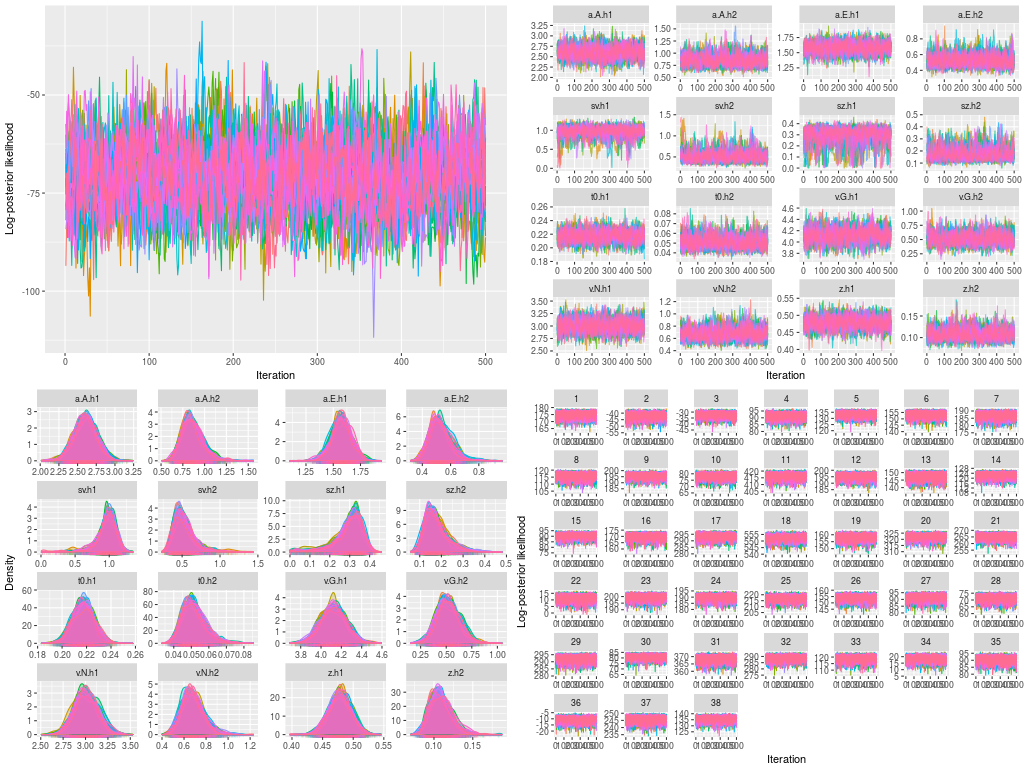
- Trace plots for the log-posterior likelihood at the hyper level
- Trace plots for hyper parameters
- Posterior density plots for the hyper parameters
- Trace plots for the log-posterior likelihood at the data level
- Posterior density plots for the DDM parameters in the 38 participants
The last figures were not presented here. They were printed separately in a pdf file for later checking.
p1 <- plot(ehsam, hyper = TRUE)
p2 <- plot(ehsam, hyper = TRUE, pll = FALSE)
p3 <- plot(ehsam, hyper = TRUE, pll = FALSE, den = TRUE)
p4 <- plot(ehsam)
p5 <- plot(ehsam, pll = FALSE, den = TRUE)
Because this is not a parameter recovery study, the next step is to estimate the DDM parameters. In the race-threshold model, we, following Pleskac, Cesario and Johson’s (2017) hypothesis, expected to see a higher threshold (at the boundary separation parameter) for a black target than for a white target. One particular strength in the hierarchical modeling is that we can ask the question that whether this specific hypothesis happens at the population level, because the hierarchical modeling assumes the 38 participants in this study are just a small subset of people the researchers (pseudo-)randomly drew from a large population, presumably the entire population in U.S.A. This is in contrast to the fixed-effect model, which assumes each participant has her / his own DDM mechanism of data generation. The following is how you may do these in ggdmc syntax.
When entering hmean = TRUE, the summary function will calculate the average values for the hyper parameters. Similarly, the option, hci = TRUE triggers the calculation of credible interval at the hyper parameters.
hest1 <- summary(hsam, hyper = TRUE, hmean = TRUE)
hest2 <- summary(hsam, hyper = TRUE, hci = TRUE)
#    a.E.h1 a.A.h1 v.G.h1 v.N.h1 z.h1 sz.h1 sv.h1 t0.h1
# h1   1.57   2.60   4.11   3.00 0.48  0.29  0.96  0.22
# h2   0.53   0.86   0.52   0.68 0.11  0.18  0.52  0.05

# Random-effect model with multiple participants
#     L 2.5%   50%   97.5% S 2.5%   50%   97.5%
# a.E   1.39  1.57    1.75   0.41  0.52    0.71
# a.A   2.32  2.60    2.89   0.67  0.85    1.14
# v.G   3.88  4.11    4.36   0.34  0.52    0.74
# v.N   2.75  3.00    3.25   0.50  0.67    0.90
# z     0.44  0.48    0.51   0.09  0.11    0.14
# sz    0.09  0.31    0.39   0.10  0.17    0.32
# sv    0.58  0.98    1.18   0.33  0.50    0.85
# t0    0.20  0.22    0.23   0.04  0.05    0.07
The results support the hypothesis that black targets result in higher decision threshold than white targets (a.E.h1 = 1.57 [1.39 - 1.75] < a.A.h1 = 2.60 [2.32 - 2.89]). Note I can make this claim because the credible intervals for these two conditions are not overlapped. Also, as expected, the drift rate for gun objects is faster than that for the non-gun objects (v.G.h1 = 4.11 [3.88 - 4.36] > v.N.h1 = 3.00 [2.75 - 3.25]). The finding of boundary separation here differs from the result in Pleskac, Cesario, & Johnson (2017, Fig. 9; also Threshold separation section on page 18). They did not find threshold difference, perhaps because they analyzed four factors, resulting in small trial numbers in each condition. I showed R codes below to print this information.
- s: subject
- S: stimulus, gun vs. nongun
- B: blur or clear object
- CT: context, danger or neutral context
- RACE: black vs. white targets
study3[, .N, .(s, S, B, CT, RACE)]
##        s   S     B     CT  RACE  N
##   1:  11 gun  blur   safe black 22
##   2:  11 non  blur   safe white 23
##   3:  11 gun clear   safe black 19
##   4:  11 non clear   safe white 18
##   5:  11 non clear   safe black 21
##  ---
## 604: 348 gun clear danger black 17
## 605: 348 non clear danger white 28
## 606: 348 gun  blur danger white 20
## 607: 348 non clear danger black 16
## 608: 348 gun  blur danger black 23
> range(study3[, .N, .(s, S, B, CT, RACE)]$N)
## [1]  6 33
In case you may be interested, I listed the estimates for each participants below. Not every participant has a higher threshold for black targets than white targets.
ests <- summary(hsam)
round(ests, 2)
##
##       a.E  a.A  v.G  v.N    z   sz   sv   t0
## 1    1.30 3.38 4.60 2.84 0.40 0.18 1.02 0.17
## 2    1.25 2.66 3.16 2.99 0.45 0.52 1.97 0.17
## 3    2.44 3.82 3.61 2.88 0.50 0.42 0.83 0.16
## 4    2.70 2.10 3.87 2.84 0.49 0.37 0.71 0.16
## 5    1.92 2.05 4.13 3.16 0.46 0.23 1.34 0.20
## 6    1.59 2.56 4.10 3.40 0.41 0.27 1.35 0.26
## 7    1.13 2.91 4.04 3.11 0.42 0.45 0.87 0.21
## 8    1.83 2.97 4.16 2.69 0.48 0.36 0.62 0.21
## 9    1.49 1.32 4.37 2.19 0.38 0.31 1.21 0.22
## 10   1.28 2.88 4.80 1.94 0.48 0.14 1.31 0.27
## 11   0.99 1.26 4.54 3.27 0.59 0.25 1.05 0.19
## 12   1.23 4.24 4.42 3.53 0.41 0.22 1.11 0.19
## 13   1.50 2.17 3.69 3.13 0.51 0.41 1.03 0.17
## 14   1.90 2.07 4.20 2.59 0.42 0.50 0.63 0.26
## 15   1.57 3.35 4.33 2.47 0.61 0.21 1.04 0.32
## 16   1.55 2.89 3.88 3.43 0.33 0.28 1.06 0.21
## 17   1.22 2.58 4.81 2.95 0.45 0.30 0.41 0.28
## 18   2.23 0.31 4.37 2.74 0.33 0.49 1.21 0.18
## 19   1.55 2.77 4.13 3.00 0.40 0.51 0.44 0.22
## 20   1.20 2.61 4.50 4.04 0.42 0.50 0.45 0.25
## 21   0.74 2.68 4.41 2.39 0.47 0.25 0.81 0.19
## 22   1.78 2.89 3.42 3.97 0.64 0.17 2.02 0.14
## 23   2.25 2.60 3.99 4.02 0.55 0.24 0.96 0.18
## 24   1.76 2.92 4.69 2.70 0.70 0.44 0.44 0.17
## 25   0.91 3.45 3.98 2.52 0.72 0.15 0.88 0.32
## 26   1.33 3.12 3.72 3.56 0.29 0.55 1.17 0.25
## 27   1.42 2.96 3.72 3.18 0.55 0.20 1.34 0.28
## 28   1.25 1.95 4.06 1.99 0.45 0.28 1.51 0.30
## 29   1.21 2.39 4.22 3.69 0.55 0.42 0.73 0.19
## 30   2.45 2.01 4.71 2.54 0.39 0.19 1.31 0.21
## 31   1.27 1.71 4.34 3.81 0.45 0.24 0.85 0.17
## 32   0.82 2.61 3.98 3.24 0.56 0.33 0.87 0.25
## 33   1.80 2.42 3.51 3.92 0.44 0.21 1.44 0.17
## 34   1.93 2.49 3.97 2.70 0.62 0.37 1.42 0.32
## 35   1.42 1.39 3.93 1.60 0.42 0.34 1.44 0.21
## 36   2.53 4.26 3.60 2.60 0.32 0.25 0.58 0.17
## 37   1.08 2.86 4.18 3.35 0.52 0.44 0.70 0.22
## 38   2.06 3.61 4.24 3.11 0.63 0.34 0.61 0.22
## Mean 1.58 2.61 4.12 3.00 0.48 0.32 1.02 0.22
Reference
Pleskac, T.J., Cesario, J. & Johnson, D.J. (2017). How race affects evidence accumulation during the decision to shoot. Psychonomic Bulletin & Review, 1-30. https://doi.org/10.3758/s13423-017-1369-6