In Bayesian computation, a prior distribution refers to a similar, but slightly different idea from the original Bayes’ theorem. I used the diffusion decisoin model (DDM, Ratcliff & McKoon, 2008) as an example to illustrate the idea.

The full DDM has eight parameters. In ggdmc (as well as DMC) syntax, they are defined as following:

p.map = list(a = “1”, v = “1”, z = “1”, d = “1”, sz = “1”, sv = “1”, t0 = “1”, st0 = “1”),

1. a: the boundary separation
2. v: the mean of the drift rate
3. z: the mean of the starting point of the diffusion relative to threshold separation
4. d: differences in the non-decisional component between upper and lower threshold
5. sz: the width of the support of the distribution of zr
6. sv: the standard deviation of the drift rate
7. t0: the mean of the non-decisional component of the response time
8. st0: the width of the support of the distribution of t0

The question is how do we determine the values for these parameters. This is where prior distribution comes in. We presume there are eight distributions jointly determine the DDM prior distribution and these eight distributions are where we draw the realized parameter values. This way, the parameter values are said stochastic, rather than deterministic. In other words, the value, for instance boundary separation, a, changes every time we consult its prior distribution. It is decided probabilistically by its prior distribution.

Below I list the full command, BuildModel, for setting up a DDM model.

## Use verbose option to suppress printing p.vector
## This is a DDM model with no manipulation factor
model <- BuildModel(
  p.map     = list(a = "1", v = "1", z = "1", d = "1", sz = "1", sv = "1",
    t0 = "1", st0 = "1"),
  match.map = list(M = list(left = "LEFT", right = "RIGHT")),
  factors   = list(S = c("left", "right")),
  constants = c(st0 = 0, d = 0),
  responses = c("LEFT", "RIGHT"),
  type      = "rd",
  verbose   = TRUE)

Set up Priors

So in this example, we will want to set up six prior distributions, because in the above model set-up, the st0 and d have been set to constant as 0. That is, they are deterministic, not stochastic. ggdmc (as well as DMC) has a function to build prior. Unimaginatively, it is called BuildPrior (it is called p.prior.dmc in DMC).

p.prior <- BuildPrior(
             p1    = c(a = 1.5, v = 3,  z = .5, sz = .3, sv = 1,  t0 = .2),
             p2    = c(a = 0.5, v = .5, z = .1, sz = .1, sv = .3, t0 =.05),
             lower = c(0, -5, 0, 0, 0, 0),
             upper = c(2, 7, 4, 4, 4, 1),
             dists = rep("tnorm", 6))

A list of options / arguments for the BuildPrior function can be found by enter:

?BuildPrior

Here is a copy from the R documentation in ggdmc pacakge.

• p1 simply means the first parameter of a distribution
• p2 simiarly mean the second parameter of a distribution
• lower is the lower support (i.e., the lower truncated boundary)
• upper is the upper support (i.e., the upper truncated boundary)
• dists is a string vector specifying the name of a distribution.

Current version of ggdmc provides four types of prior distributions:

1. tnorm, Normal and truncated normal, where: p1 = mean, p2 = sd. It specifies a normal distribution when bounds are set -Inf and Inf,
2. beta, Beta, where: p1 = shape1 and p2 = shape2 (see ?pbeta in R). Note the uniform distribution is a special case of the beta distribution when p1 and p2 = 1,
3. gamma, Gamma, where p1 = shape and p2 = scale (see ?pgamma in R). Note p2 is scale, not rate,
4. lnorm, Lognormal, where p1 = meanlog and p2 = sdlog (see ?plnorm).

In the ggdmc (as well as DMC) operation, the names (i.e., character strings) are important for corret computation.

The two options, lower and upper, are to set the distribution support.

• for tnorm, these define the lower and upper bounds; When the user enters NA , the default behaviour of the function is to set the values as -Inf and Inf. This make a truncated normal distribution becoming a normal distribution (see ?pnorm).
• for beta, these define the lower and upper bounds (i.e., scaled beta distribution). The default behaviour for entering NA is to filled with the values of 0 and 1.
  • p1 = 1 & p2 = 1 & lower = 0 (default) & upper = 1 (default) creates Uniform(0, 1)
  • p1 = 1 & p2 = 1 & lower = l & upper = u creates Uniform(l, u)
• for gamma, lower shifts the distribution to exclude small values
• for lognormal, lower shifts the distribution to exclude small values

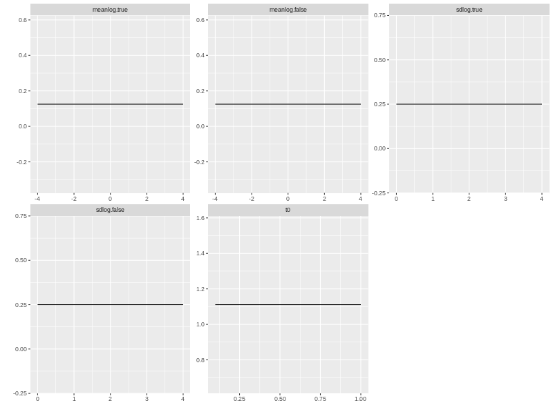
Example 1: Set up beta (and uniform) prior

Currently, the below example is from Heathcote et al’s (2018) DMC tutorial of LNR model.

beta.prior <- BuildPrior(
  dists = c("beta", "beta", "beta", "beta", "beta"),
  p1 = c(meanlog.true = 1, meanlog.false = 1, sdlog.true = 1, sdlog.false = 1, t0 = 1),
  p2 = c(meanlog.true = 1, meanlog.false = 1, sdlog.true = 1, sdlog.false = 1, t0 = 1),
  lower = c(-4,-4, 0, 0, 0.1),
  upper = c( 4, 4, 4, 4, 1))

You can plot and print the prior distribution by using the plot and print functions.

plot(beta.prior)

print(p.prior)

##               p1 p2 lower upper log    dist  untrans
## meanlog.true   1  1    -4     4   1 beta_lu identity
## meanlog.false  1  1    -4     4   1 beta_lu identity
## sdlog.true     1  1     0     4   1 beta_lu identity
## sdlog.false    1  1     0     4   1 beta_lu identity
## t0             1  1   0.1     1   1 beta_lu identity

This is how to calculate log-prior likelihoods (i.e., probability densities) for each model parameter and add them all together.

dprior(p.vector, p.prior)

## meanlog.true meanlog.false    sdlog.true   sdlog.false            t0 
##    -2.0794415    -2.0794415    -1.3862944    -1.3862944     0.1053605

sumlogpriorNV(p.vector, p.prior)

## [1] -6.826111

What to look for when set up prior distributions

For setting up prior distributions, key points are to look for first whether prior distributions cover broad range (i.e., relatively uninformative) and second whether their range cover abnormal values. For example, it is not possible to have negative standard devation, so sd_v.true subpanel should not cover negative values.