In this tutorial, I illustrated fitting multiple participants, assuming the mechanism of data generation is fixed-effect models. That is, each participant is accounted for by independent mechanisms. I also assume the LBA model is the true RT model.
I made up a two-factor factorial design. The first two-level factor is the stimulus (S). Suppose the stimuli have two types: one is low quality face photos, so people find it hard to recognize and the other is normal quality face photo. The second factor is the frequency (F), supposing one type is the celebrity photos, so people perhaps see more often, and the other is the photos of randomly selected strangers.
In the model set-up, I presume a rate model, which has its drift rates affected by the two factors, S and F. The latent factor, M, is just a LBA way to model independent accumulators. Another factor, R, not explicitly in the factorial design, is an indicator factor, indicating the response type affecting the threshold parameter (i.e., accumulators traveling distance).
require(ggdmc)
model <- BuildModel(
          p.map     = list(A = "1", B = "R", t0 = "1",
            mean_v = c("S", "F", "M"), sd_v = "M", st0 = "1"),
          match.map = list(M = list(s1 = 1, s2 = 2)),
          factors   = list(S = c("s1", "s2"), F = c("f1", "f2")),
          constants = c(sd_v.false = 1, st0 = 0),
          responses = c("r1", "r2"),
          type      = "norm")
##  [1] "A"                  "B.r1"               "B.r2"
##  [4] "t0"                 "mean_v.s1.f1.true"  "mean_v.s2.f1.true"
##  [7] "mean_v.s1.f2.true"  "mean_v.s2.f2.true"  "mean_v.s1.f1.false"
## [10] "mean_v.s2.f1.false" "mean_v.s1.f2.false" "mean_v.s2.f2.false"
## [13] "sd_v.true"
npar <- length(GetPNames(model))
To simulate many participants, I set up a population distribution, which is not in line with the assumption of fixed-effects model. That is, this way to generate data is to presume that a random-effects model at work. For the purpose of illustration, I forgo this issue for now.
pop.mean <- c(A = .4, B.r1 = .85, B.r2 = .8, t0 = .1,
              mean_v.s1.f1.true = 2.5,    mean_v.s2.f1.true = 3.5,
              mean_v.s1.f2.true = 4.5,    mean_v.s2.f2.true = 5.5,
              mean_v.s1.f1.false = 1.00,  mean_v.s2.f1.false = 1.10,
              mean_v.s1.f2.false = 1.05,  mean_v.s2.f2.false = 1.20,
              sd_v.true = .25)
pop.scale <- c(A = .1, B.r1 = .1, B.r2 = .1, t0 = .05,
              mean_v.s1.f1.true = .2,   mean_v.s2.f1.true = .2,
              mean_v.s1.f2.true = .2,   mean_v.s2.f2.true = .2,
              mean_v.s1.f1.false = .2,  mean_v.s2.f1.false = .2,
              mean_v.s1.f2.false = .2,  mean_v.s2.f2.false = .2,
              sd_v.true = .1)

pop.prior <- BuildPrior(
  dists = rep("tnorm", npar),
  p1    = pop.mean,
  p2    = pop.scale,
  lower = c(rep(0, 4), rep(NA, 8), 0),
  upper = c(rep(NA, npar)))
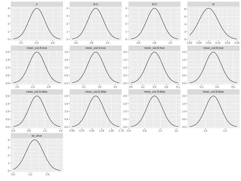
We may want to check how the prior distributions look like. ggdmc has a plot function to do just that. Note you need to load ggdmc package (i.e., require(ggdmc)) to make plot function changes its default behaviour.
plot(pop.prior)
## Simulate some data
dat <- simulate(model, nsim = 30, nsub = 8, prior = pop.prior)
dmi <- BuildDMI(dat, model)
dplyr::tbl_df(dat)
## # A tibble: 960 x 5
##    s     S     F     R        RT
##    <fct> <fct> <fct> <fct> <dbl>
##  1 1     s1    f1    r1    0.438
##  2 1     s1    f1    r1    0.517
##  3 1     s1    f1    r1    0.407
##  4 1     s1    f1    r1    0.454
##  5 1     s1    f1    r1    0.449
##  6 1     s1    f1    r1    0.463
##  7 1     s1    f1    r1    0.552
##  8 1     s1    f1    r1    0.411
##  9 1     s1    f1    r1    0.387
## 10 1     s1    f1    r1    0.486
## # ... with 950 more rows
The true averaged parameter vectors, which were randomly chosen based on pop.prior, can be retrieved by looking up the parameters attribute, attached onto the dat object. However, note the real true values are pop.mean and pop.scale, because the data are generated based on random-effects model.
require(matrixStats)
ps <- attr(dat, "parameters")
mu <- round(colMeans2(ps), 2)
sigma <- round(colSds(ps), 2)
truevalues <- rbind(mu, sigma)
colnames(truevalues) <- GetPNames(model)


## Set up prior distributions
p.prior <- BuildPrior(
  dists = rep("tnorm", npar),
  p1    = pop.mean,
  p2    = pop.scale*20,
  lower = c(rep(0, 4), rep(NA, 8), 0),
  upper = c(rep(NA, npar)))
Now we am ready to fit the eight participants. Ideally, this can be done simultaneously, if a eight-core machine is available. Here I used a four-core machine so launched 2 cores only (ncore = 2).
## Sampling -------------
fit0 <- StartNewsamples(dmi, p.prior, ncore = 2)
fit  <- run(fit0, 5e2, ncore = 2)
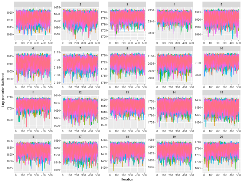
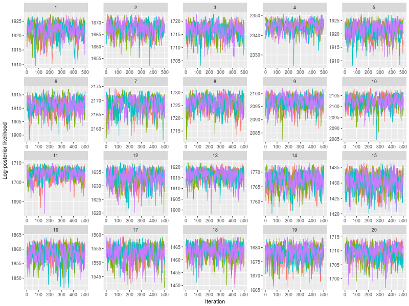
Use plot to check whether posterior log-likelihood converged.
plot(fit)
gelman function prints the potential scale reduction factor (psrf). A psrf value less than 1.1 suggests chains are well-mixed.
res <- gelman(fit, verbose = TRUE)
# Diagnosing theta for many participants separately
#   15   20   13   18    6   17   12   19    5   11    8    3   16   14    1    2    9
# 1.01 1.01 1.01 1.01 1.01 1.01 1.01 1.01 1.01 1.01 1.01 1.01 1.01 1.01 1.01 1.02 1.02
#    4    7   10
# 1.02 1.03 1.03
# Mean
# [1] 1.01
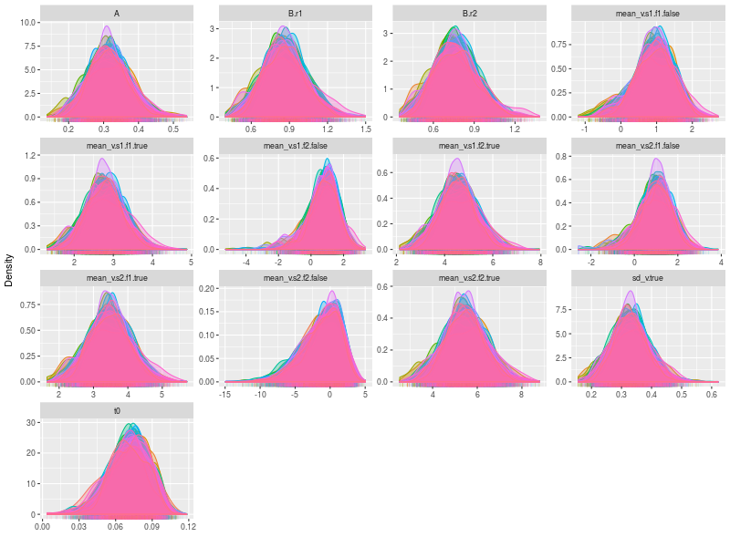
By setting the option, pll (posterior log-likelihood), to FALSE and the option, den (density plot), to TRUE , we can check the trace plots for each model parameters. Because there are several participants, the size of the figure is considerably large. It may be a better to plot separately in a pdf file and check it later.
pdf("figs/subjects-density.pdf")
lapply(fit, ggdmc:::plot.model, pll = FALSE, den = TRUE )
dev.off()
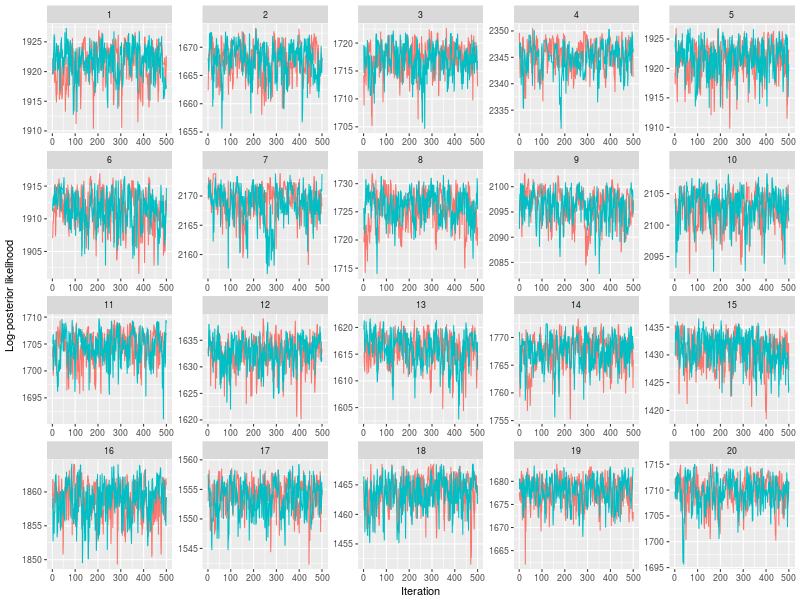
One specific feature in ggdmc is that it uses pMCMC, so occasionally, we want to check a subset of chains. The function will randomly pick three chains to plot
plot(sam, subchain = TRUE)
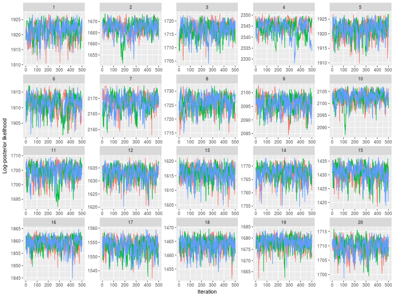
You can indicate how many subset of chains to plot, too.
plot(sam, subchain = TRUE, nsubchain = 4))
You can also indicate which chains, instead of randomly selecting a subset of chains.
plot(sam, subchain = TRUE, nsubchain = 4, chains = c(1:4))
These are a lot of checks! Finally and fortunately, because this is a parameter recovery study, I can look up the true parameters to see if I do estimate them well. summary function will do the trick by entering TRUE for the recovery option and entering the true parameter matrix, which I had stored it to a ps object before, to ps option.
est <- summary(sam, recovery = TRUE, ps = ps)
# Summary each participant separately
#          A  B.r1  B.r2    t0 mean_v.s1.f1.true mean_v.s2.f1.true mean_v.s1.f2.true
# Mean  0.50  1.02  0.96  0.10              3.05              4.34              5.50
# True  0.41  0.82  0.77  0.10              2.49              3.56              4.50
# Diff -0.09 -0.20 -0.19  0.00             -0.56             -0.78             -1.00

# Sd    0.15  0.20  0.17  0.05              0.49              0.44              0.76
# True  0.11  0.10  0.09  0.05              0.21              0.19              0.22
# Diff -0.04 -0.10 -0.08 -0.01             -0.28             -0.25             -0.54
#      mean_v.s2.f2.true mean_v.s1.f1.false mean_v.s2.f1.false mean_v.s1.f2.false
# Mean              6.69               1.59               1.58               0.70
# True              5.49               1.03               1.15               1.08
# Diff             -1.20              -0.56              -0.43               0.38

# Sd                0.82               0.34               1.21               1.58
# True              0.22               0.15               0.23               0.15
# Diff             -0.59              -0.19              -0.98              -1.43
#      mean_v.s2.f2.false sd_v.true
# Mean              -0.38      0.30
# True               1.11      0.24
# Diff               1.48     -0.06

# Sd                 1.23      0.11
# True               0.16      0.10
# Diff              -1.07     -0.01