Disclaimer: This tutorial uses an experimental (beta) version of ggdmc, which has added the functionality of fitting logistic regression models. The software can be found in its GitHub. This document has yet completed.
The aim of tutorial is to document one method to fit the logistic regression model, using the Seeds data. Seeds data were studied in Crowder (1978), re-analysed by Breslow and Clayton (1993) and used in the BUGS examples volumn I. This document expands the scope of ggdmc to the logistic regression model.
An ordinary logistic model can fit either binary (response) data (i.e., 0, 1, 0, …) or binomial data (i.e., proportional data, as the Seeds example). The simplest form of the random-effect (multilevel) logistic model is to presume observation units are drawn from a normal distribution.
\[\begin{align*} & y_i \sim Binomial(p_i, n_i) \\ & p_i = logit^{-1}(\mathbf{X} \beta + s_i) \\ & s_i \sim N(0, \sigma^2) \end{align*}\]This two-level model can be compared to the model presuming observation units are as they been observed (i.e., fixed-effect logistic regression model).
\[\begin{align*} & y_i \sim Binomial(p_i, n_i) \\ & p_i = logit^{-1}(\mathbf{X} \beta) \\ \end{align*}\]Here I use the formulation of anti-logit, because firstly it is easier to interpret the probability of success (i.e., \(p_i\)) and secondly it is practically how computer codes been implemented. The idea of transforming binary or binomial responses with logit is still conceptually important for the generalized linear model though.
\[\begin{align*} & logit(p_i) =\mathbf{X} \beta \\ \end{align*}\]Because the Seeds data set was formatted as List, I convert the data to data frame format.
rm(list = ls())
library(data.table); library(boot)
## Load Seeds data ------------
## 2 x 2 design
setwd("~/BUGS_Examples/vol1/Seeds/")
dat <- list(S = c(10, 23, 23, 26, 17,  5, 53, 55, 32, 46,
                  10,  8, 10,  8, 23,  0,  3, 22, 15, 32,
                  3),
            N = c(39, 62, 81, 51, 39,  6, 74, 72, 51, 79,
                  13, 16, 30, 28, 45,  4, 12, 41, 30, 51,
                  7),
            ## seed variety; 0 = aegytpiao 75 1 = aegyptiao 73
            X1 = c(0, 0, 0, 0, 0,  0, 0, 0, 0, 0,
                   0, 1, 1, 1, 1,  1, 1, 1, 1, 1,
                   1),
            ## root extract; 0 = bean; 1 = cucumber
            X2 = c(0, 0, 0, 0, 0,  1, 1, 1, 1, 1,
                   1, 0, 0, 0, 0,  0, 1, 1, 1, 1,
                   1),
            Ns = 21)

d <- data.table(S = dat$S, N = dat$N, P = dat$S/dat$N, X1= dat$X1, X2 = dat$X2)
dplyr::tbl_df(d)
d$s <- factor(1:dat$Ns)
## A tibble: 21 x 7
##        S     N     P    X1    X2   logit s
##    <dbl> <dbl> <dbl> <dbl> <dbl>   <dbl> <fct>
##  1    10    39 0.256     0     0 -1.06   1
##  2    23    62 0.371     0     0 -0.528  2
##  3    23    81 0.284     0     0 -0.925  3
##  4    26    51 0.510     0     0  0.0392 4
##  5    17    39 0.436     0     0 -0.258  5
##  6     5     6 0.833     0     1  1.61   6
##  7    53    74 0.716     0     1  0.926  7
##  8    55    72 0.764     0     1  1.17   8
##  9    32    51 0.627     0     1  0.521  9
## 10    46    79 0.582     0     1  0.332  10
## ... with 11 more rows
- S, the number of (successfully) germinated seeds on the ith plate (i = 1, … N);
- N, the number of total seeds on the ith plate;
- P, the proportion of germinated seeds;
- X1, a two-level seed factor, aegyptiao 75 vs. aegyptiao 73;
- X2, a two-level root extract factor, bean vs. cucumber;
- logit, as the column name says;
- s, subject, namely, the observation unit.
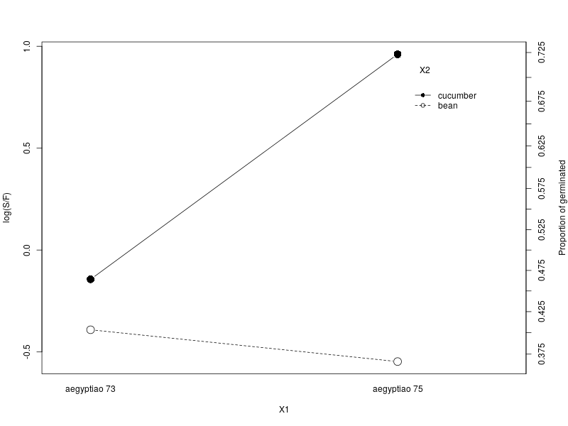
The interaction plot shows that the root extract type, cucumber, has a drastic increase in successful germination when the seed type is aegyptiao 75, comparing to when the seed type is aegyptaio 73 and this change is small and in an opposite direction in the root extract type, bean.
The data can be analysed with the ordinary logistic regression (OLR) model or multilevel logistic regression model. The OLR replicates the result in Table 3 (1st column) in Breslow and Clayton (1993). I use the display function in the arm package, which shows summary result concisely (AIC is calculated separately).
m1 <- glm(cbind(S, N-S) ~ X1 + X2, family = binomial, data = d)
arm::display(m1)
## Breslow's result in Table 3 p15
## glm(formula = cbind(S, N - S) ~ X1 + X2, family = binomial, data = d)
##             coef.est coef.se
## (Intercept) -0.43     0.11
## X1          -0.27     0.15
## X2           1.06     0.14
## ---
## n = 21, k = 3
## residual deviance = 39.7, null deviance = 98.7 (difference = 59.0)
## AIC: 122.28


m2 <- glm(cbind(S, N-S) ~ X1*X2, family = binomial, data = d)
arm::display(m2)
## glm(formula = cbind(S, N - S) ~ X1 * X2, family = binomial, data = d)
##             coef.est coef.se
## (Intercept) -0.56     0.13
## X1           0.15     0.22
## X2           1.32     0.18
## X1:X2       -0.78     0.31
## ---
## n = 21, k = 4
## residual deviance = 33.3, null deviance = 98.7 (difference = 65.4)
## AIC: 117.87

require(lme4)
m3 <- glmer(cbind(S, N - S) ~ X1 * X2 + (1 | s), family = binomial(link="logit"), data = d)
arm::display(m3)
## glmer(formula = cbind(S, N - S) ~ X1 * X2 + (1 | s), data = d,
##       family = binomial(link = "logit"))
##          coef.est coef.se
## (Intercept) -0.55     0.17
## X1           0.10     0.28
## X2           1.34     0.24
## X1:X2       -0.81     0.38
##
## Error terms:
## Groups   Name        Std.Dev.
## s        (Intercept) 0.23
## Residual             1.00
## ---
## number of obs: 21, groups: s, 21
## AIC = 117.5, DIC = -74.6
## deviance = 16.5
| glm | glmer | BUGS | ggdmc | |||||
|---|---|---|---|---|---|---|---|---|
| \(\beta\) | se | \(\beta\) | se | \(\beta\) | se | \(\beta\) | se | |
| \(\alpha_0\) | -0.558 | 0.126 | -0.548 | 0.166 | -0.557 | 0.197 | ||
| \(\alpha_{1}\) | 0.146 | 0.223 | 0.097 | 0.277 | 0.086 | 0.317 | ||
| \(\alpha_{2}\) | 1.318 | 0.177 | 1.337 | 0.236 | 1.348 | 0.276 | ||
| \(\alpha_{12}\) | -0.778 | 0.306 | -0.810 | 0.384 | -0.824 | 0.445 | ||
| \(\sigma\) | — | — | 0.235 | — | 0.286 | 0.146 |