We have striven to minimize the number of errors. However, we canot guarantee the note is 100% accurate.
In this tutorial, I conducted a parameter recovery study, demonstrating the pMCMC method to fit a hierarchical DDM for a relatively simple factorial design.
Set-up a model object
This particular design is from Heathcote et al’s (2018) DMC tutorial, which assumes a word frequency (my interpretation) factor affecting the mean drift rate (v). Note it is not a good practice to use “F” notation in R, because it is also used as a shorthand for the reserved word, meaning FALSE. However, one of the R strengths is it permits idiosyncratic programming habits, even bad ones. In the example here, it seems not cause any errors.
## version 0.2.6.0
## install.packages("ggdmc")
loadedPackages <-c("ggdmc", "data.table", "ggplot2", "gridExtra", "ggthemes")
sapply(loadedPackages, require, character.only=TRUE)

model <- BuildModel(
    p.map     = list(a = "1", v = "F", z = "1", d = "1", sz = "1", sv = "1",
                     t0 = "1", st0 = "1"),
    match.map = list(M = list(s1 = "r1", s2 = "r2")),
    factors   = list(S = c("s1", "s2"), F = c("f1", "f2")),
    constants = c(st0 = 0, d = 0),
    responses = c("r1", "r2"),
    type      = "rd")
npar <- length(GetPNames(model))
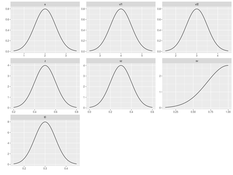
To conduct a parameter recovery study, I firstly assumed a hidden multi-level mechanism generating the data. That is, I presumed there is a distribution at the population / participants level. This distribution is a 7 dimension distribution, which has 7 marginal distributions. Each of them is in control of one DDM parameter.
pop.mean  <- c(a = 2,  v.f1 = 4, v.f2 = 3,  z = .5, sz = .3, sv = 1,  t0 = .3)
pop.scale <- c(a = .5, v.f1 =.5, v.f2 = .5, z = .1, sz = .1, sv = .3, t0 = .05)
pop.prior <- BuildPrior(
   dists = rep("tnorm", npar),
   p1    = pop.mean,
   p2    = pop.scale,
   lower = c(0, rep(-5, 2), rep(0, 4)),
   upper = c(5, rep( 7, 2), 1, 2, 1, 1))
As usual, I want to visually check if the assumed mechanism is reasonable.
plot(pop.prior)
After making sure that the data generating mechanism is proper, I then simulated a data set with 40 participants and 250 trials for each condition.
dat <- simulate(model, prior = pop.prior, nsim = 250, nsub = 40)
dmi <- BuildDMI(dat, model)
ps  <- attr(dat, "parameters")
In the hierarchical case of the parameter recovery study, my aim is to recover not only ps matrix, but also the data generating mechanism. That is, I also want to known pop.mean, pop.scale and their marginal distribution. Note ps is a matrix, storing the true values for each DDM parameter. That is, the simulate function randomly selects nsub set of true parameters based on the prior distribution, pop.prior. Each row of the ps matrix represents one parameter vector of a participant.
tibble::as_tibble(ps)
## A tibble: 40 x 7
##        a  v.f1  v.f2     z    sz    sv    t0
##    <dbl> <dbl> <dbl> <dbl> <dbl> <dbl> <dbl>
##  1  2.93  4.30  2.95 0.486 0.151 0.775 0.304
##  2  1.52  3.74  2.40 0.589 0.258 0.809 0.340
##  3  1.85  4.31  2.62 0.636 0.318 0.903 0.349
##  4  2.34  3.94  2.53 0.578 0.127 0.993 0.283
##  5  2.44  4.50  2.68 0.566 0.246 0.589 0.261
##  6  2.73  4.08  3.68 0.465 0.182 0.973 0.290
##  7  2.34  2.89  3.69 0.742 0.307 0.592 0.325
##  8  1.90  4.35  3.56 0.512 0.186 0.513 0.309
##  9  2.60  4.18  2.81 0.541 0.367 0.758 0.270
## 10  1.64  3.77  2.37 0.596 0.286 0.995 0.375
##  with 30 more rows
The above is only preparation work for a parameter recovery study. In the following, I will start to draw samples from the posterior distribution, aiming to recover pop.mean, pop.scale, the target distribution, and the ps matrix.
I already have the likelihood, which is the DDM equation (Voss, Rothermund, Voss, 2004). I will need to set up the prior distributions for the seven DDM parameters. In the case of hierarchical model, there are two sets of prior distributions: one is usually called hyper-prior distributions and the other simply prior distributions. The former is my prior belief about the distributions (pp.prior below) accounted by pop.mean and pop.scale. The latter is my prior belief about separate DDM mechanisms for each individual participant (p.prior below).
p.prior <- BuildPrior(
  dists = rep("tnorm", npar),
  p1    = pop.mean,
  p2    = pop.scale*5,
  lower = c(0,-5, -5, rep(0, 4)),
  upper = c(5, 7,  7, 1, 2, 1, 1))
mu.prior <- BuildPrior(
  dists = rep("tnorm", npar),
  p1    = pop.mean,
  p2    = pop.scale*5,
  lower = c(0,-5, -5, rep(0, 4)),
  upper = c(5, 7,  7, 1, 2, 1, 1))
sigma.prior <- BuildPrior(
  dists = rep("beta", npar),
  p1    = rep(1, npar),
  p2    = rep(1, npar),
  upper = rep(2, npar))

names(sigma.prior) <- GetPNames(model)
A convention in ggdmc is to bind location and scale prior distributions as one list object. This is just for the convenience of data handling in R, which is not so convenient in C++. Note the names of each element in the list is critical.
priors <- list(pprior = p.prior, locaton = mu.prior, scale = sigma.prior)
Then, the following run sampling.
## run the "?" to see the details of function options
?StartNewsamples
?run
## 7.84 mins
fit0 <- StartNewsamples(data=dmi, prior=priors)

## 19 mins
fit <- run(fit0)

## 7.54 hrs
fit <- run(fit, thin = 8)

save(pop.mean, pop.scale, pop.prior, model, dat, dmi, npar, ps,
     fit0, fit, file = "data/hierarchical/ggdmc_4_7_DDM.rda")
One may use the repeat function to run automatic model fit.
## 4 rounds
thin <- 8
repeat {
     hsam <- run(RestartHypersamples(5e2, hsam, thin = thin),
                 pm = 0, hpm = 0)
     save(pop.mean, pop.scale, pop.prior, model, dat, dmi, npar, ps,
          hsam0, hsam, file = "data/hierarchical/ggdmc_4_7_DDM.rda")
     rhats <- hgelman(hsam)
     thin <- thin * 2
     if (all(rhats < 1.1)) break
}

save(pop.mean, pop.scale, pop.prior, model, dat, dmi, npar, ps,
  hsam0, hsam, file = "data/hierarchical/ggdmc_4_7_DDM.rda")
Similar to many standard modeling works, I must diagnose the model fit to certain I drew a reliable posterior distribution, reflecting the target distribution. I can check visually as well as calculate some statistics. First, I conducted visual checks for the trace plots and posterior distributions.
- Trace plots of posterior log-likelihood at hyper level
- Trace plots of the hyper parameters
- Trace plots of posterior log-likelihood at the data level
- Trace plots of each DDM parameters for each participants
- Posterior density plots (i.e., marginal posterior distributions) for the hyper parameters
- Posterior density plots of each DDM parameters at the data level
plot(hsam, hyper = TRUE)                           ## 1.
plot(hsam, hyper = TRUE, pll = FALSE)              ## 2.
plot(hsam)                                         ## 3.
plot(hsam, pll = FALSE)                            ## 4.
plot(hsam, hyper = TRUE, pll = FALSE, den = TRUE)  ## 5.
plot(hsam, pll = FALSE, den = TRUE)                ## 6.
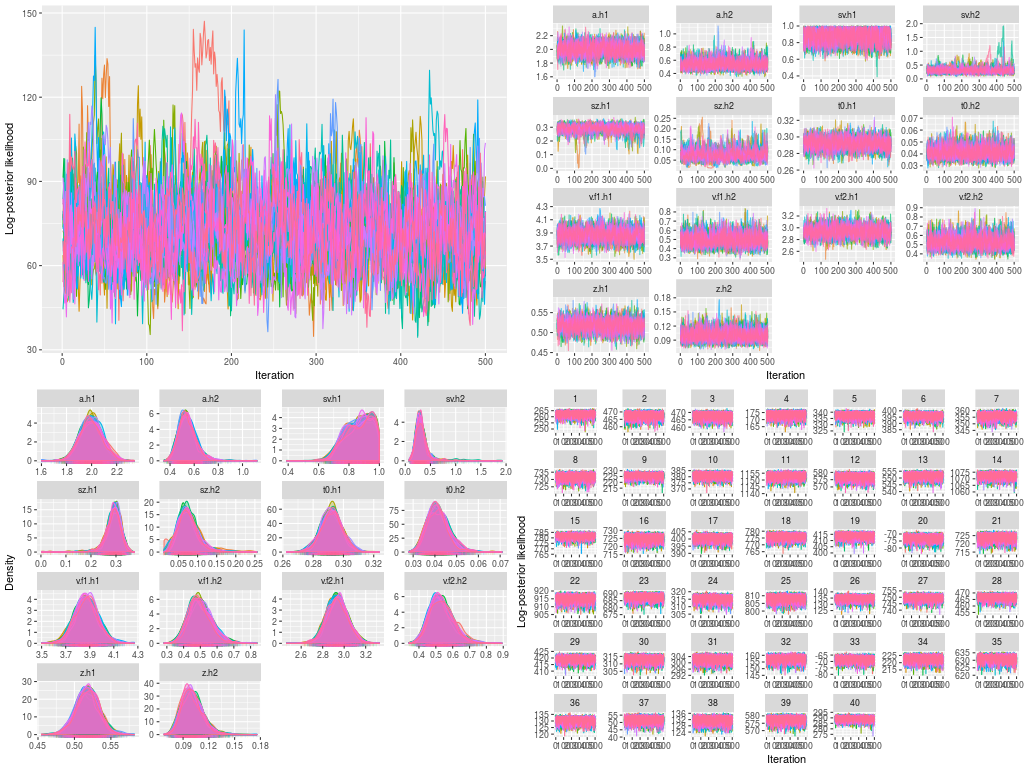
These are a lot of figures to check. I have not presented the figures of posterior probability density for every participant (i.e., figure 6), because there are too many. You can print them in a pdf file to check.
Then, I calculated the potential scale reduction factor, for both the hyper parameters and the parameters for each participant.
rhats <- hgelman(hsam, verbose = TRUE)
## Diagnosing theta for many participants separately
## Diagnosing the hyper parameters, phi
## hyper     1     2     3     4     5     6     7     8     9    10    11    12
##  1.02  1.00  1.00  1.00  1.00  1.00  1.00  1.00  1.00  1.00  1.00  1.00  1.00
##    13    14    15    16    17    18    19    20    21    22    23    24    25
##  1.00  1.00  1.00  1.00  1.00  1.00  1.00  1.00  1.00  1.00  1.00  1.00  1.00
##    26    27    28    29    30    31    32    33    34    35    36    37    38
##  1.00  1.00  1.00  1.00  1.00  1.00  1.00  1.00  1.00  1.00  1.00  1.00  1.00
##    39    40
##  1.01  1.01
Finally, I want to know if I do recover the data generation mechanism and true parameter values for every participant (i.e., ps). This can be achieved by using the summary function.
hest1 <- summary(hsam, recovery = TRUE, hyper = TRUE, ps = pop.mean,  type = 1)
hest2 <- summary(hsam, recovery = TRUE, hyper = TRUE, ps = pop.scale, type = 2)
round(hest1, 2)
round(hest2, 2)
ests <- summary(hsam, recovery = TRUE, ps = ps)

##                   a    sv    sz    t0  v.f1  v.f2    z
## True           2.00  1.00  0.30  0.30  4.00  3.00 0.50
## 2.5% Estimate  1.83  0.69  0.22  0.28  3.69  2.76 0.49
## 50% Estimate   2.00  0.88  0.29  0.29  3.87  2.93 0.52
## 97.5% Estimate 2.17  0.99  0.34  0.31  4.07  3.12 0.55
## Median-True    0.00 -0.12 -0.01 -0.01 -0.13 -0.07 0.02

##                   a   sv    sz    t0  v.f1 v.f2    z
## True           0.50 0.30  0.10  0.05  0.50 0.50 0.10
## 2.5% Estimate  0.43 0.15  0.03  0.03  0.38 0.41 0.08
## 50% Estimate   0.53 0.30  0.07  0.04  0.49 0.53 0.10
## 97.5% Estimate 0.71 0.58  0.14  0.05  0.65 0.68 0.13
## Median-True    0.03 0.00 -0.03 -0.01 -0.01 0.03 0.00


## Summary statistics across participants
##          a  v.f1 v.f2    z    sz   sv   t0
## Mean  2.00  3.87 2.94 0.52  0.29 0.72 0.29
## True  1.98  3.86 2.94 0.52  0.28 0.78 0.29
## Diff -0.02 -0.01 0.00 0.00 -0.01 0.06 0.00
## Sd    0.51  0.44 0.49 0.10  0.04 0.15 0.04
## True  0.52  0.47 0.51 0.10  0.09 0.19 0.04
## Diff  0.00  0.02 0.02 0.00  0.05 0.04 0.00