This is a short note for one method to conduct maximum likelihood estimation (MLE) to fit the LBA model.
In essence, the MLE is not a very difficult statistical technique, but there are some trivialities regarding to the cognitive model and its influence on the usage of optimiser that must be addressed. Otherwise, you would not recover the parameters in the LBA model (or cognitive models in general).
In short, you must adjust either the objective function, the method of data preparation, or the method of proposing parameters according to a specific cognitive model. For example, the non-decision time must not go below 0 second. If you do not (or cannot) add this constraint on the optimiser (e.g., the R function, optim), the resulting fit may not converge or the estimates (even converged) will be unreasonable, psychologically speaking.
Below I use ggdmc to conduct a simulation study to demonstrate the point.
Simulation study
Firstly, I use the BuildModel function to set up a null model with only a stimulus factor (denoted S). That is, the model parameters do not associate with any factors.
Next I arbitrarily set up a true parameter vector, p.vector and request 100 trials per condition. My aim is to recover the true parameters.
require(ggdmc)
model <- BuildModel(
  p.map     = list(A = "1", B = "1", t0 = "1", mean_v = "M", sd_v = "1",
                   st0 = "1"),
  match.map = list(M = list(s1 = 1, s2 = 2)),
  factors   = list(S = c("s1", "s2")),
  constants = c(st0 = 0, sd_v = 1),
  responses = c("r1", "r2"),
  type      = "norm")

p.vector <- c(A = .75, B = 1.25, t0 = .15, mean_v.true = 2.5, mean_v.false = 1.5)
ntrial <- 1e2

## I used the seed option to make sure I always replicate the result.
dat <- simulate(model, nsim = ntrial, ps = p.vector, seed = 123)
dmi <- BuildDMI(dat, model)
Description statistics
As a good practice, we check some basic descriptive statistics. Here is the response time distributions, drawn as one correct RT and one error RT histograms.
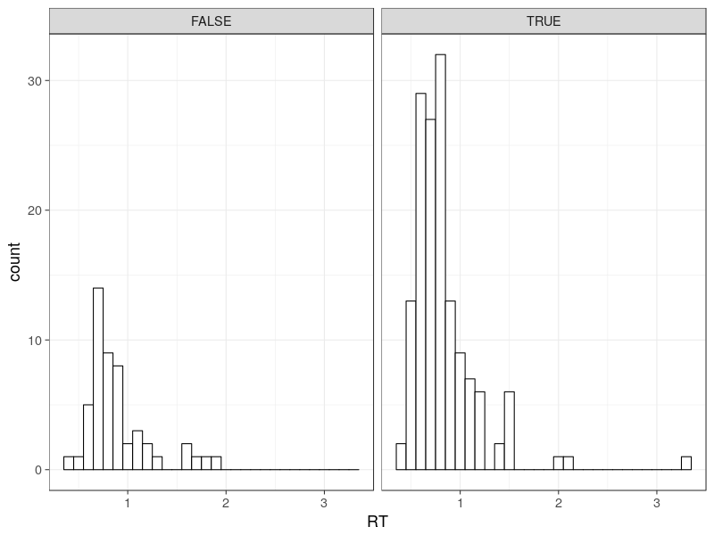
Note there are two histograms (i.e., distributions). This is one of the specific feature in the choice RT models. This is sometimes dubbed defective distributions, meaning multiple distributions jointly composing a complete model (integrated to 1).
The likelihood function in the ggdmc has considered this, so you will not see how the internal C++ codes handle this triviality. But if you use the bare-bones LBA density functions, say “ggdmc:::n1PDFfixedt0” (meaning node 1 probability density function), “ggdmc:::fptcdf” or “ggdmc:::fptpdf”, you need to handle the calculation of “defective distributions” accordingly. These are the functions originally from Brown and Heathcote(2008), but since version 0.2.6.7, ggdmc has no longer exposed them in R interface.
By the way, the top x axis in the above figure labels TRUE, representing correct responses and FALSE, representing error responses. It is not unusual to observe more correct responses than error responses, so the simulation produces realistic data.
Since version 0.2.7.6, ggdmc uses S4 class to replace original informal S3 class. So the data is now stored as a slot in the dmi object.
## This is to create a column in the data frame to indicate
## correct and error responses.
dmi@data$C <- ifelse(dmi@data$S == "s1" & dmi@data$R == "r1", TRUE,
              ifelse(dmi@data$S == "s2" & dmi@data$R == "r2", TRUE,
              ifelse(dmi@data$S == "s1" & dmi@data$R == "r2" ,FALSE,
              ifelse(dmi@data$S == "s2" & dmi@data$R == "r1", FALSE, NA))))

prop.table(table(dmi@data$C))
## FALSE == error responses (25.5%)
## TRUE == correct responses (74.5%)
## FALSE  TRUE
## 0.255 0.745

## The maximum (log) likelihoods
##
den <- likelihood(p.vector, dmi)
sum(log(den))
## [1] -112.7387
Maximum likelihood estimation
The following is the objective function. Note data must be a data model instance. This requirement is to use ggdmc internal to handle many trivialities, for instance, the defective distributions, experimental design, transforming parameter (\(b = A + B\)), etc. If you use the bare-bones density functions, you must handle these trivialities. Also I use negative log likelihood.
objective_fun <- function(par, data) {
  ## Internally, C++ likelihood function will read model type, and
  ## new Likelihood constructor (in Likelihood.hpp) will read S4 slot.
  ## So here data variable is OK to be a data-model instance
  den <- likelihood(par, data)
  return(-sum(log(den)))
}
init_par[3] <- runif(1, 0, min(dmi$RT))
This line makes starting non-decision time not less than the minimal RT in the data. This is another psychological consideration. It may help. However, it does not guarantee the optimiser won’t propose a non-decision time less than minimal RT in the data.
init_par <- runif(5)
init_par[3] <- runif(1, 0, min(dmi@data$RT))
names(init_par) <- c("A", "B", "t0", "mean_v.true", "mean_v.false")
res <- nlminb(objective_fun, start = init_par, data = dmi, lower = 0)
round(res$par, 2)  ## remember to check res$convergence
Below is a list of possible estimates. The last line show the true parameter vector for the convenience of comparison. The first column shows the numbers of trial per condition. At the size of 1e5, the recovered values almost equal to the true values.
##         A       B      t0 mean_v.true mean_v.false
## 1e2  0.79    0.98    0.17   2.26      0.77
## 1e2  0.86    1.74    0.04   2.80      1.82
## 1e2  0.91    0.67    0.28   2.04      1.02
## 1e2  0.72    1.36    0.14   2.74      1.60
## 1e3  0.71    1.15    0.16   2.32      1.40
## 1e3  0.61    1.63    0.08   2.70      1.76
## 1e4  0.71    1.28    0.15   2.51      1.50
## 1e5  0.75    1.24    0.15   2.49      1.49
## true 0.75    1.25    0.15   2.50      1.50
Instead of using the optim function, I opt to nlminb function. This is again a model specific consideration. In the LBA model, A, B, and t0 must not be less than 0, so it will help if we can impose this constraint. Both optim and nlminb offer an argument, lower, to constraint the parameter proposals. However, if you impose the lower constraint, optim allows only (?) the optimisation method, “L-BFGS-B”, which does not handle well infinite. Unfortunately, in fitting the LBA model, it is likely some parameter proposals result in infinite log-likelihoods.
Bonus
A better way to initialise a parameter proposal is to use prior distributions. rprior in ggdmc allows you to easily do this. This is a step towards Bayesian.
p.prior <- BuildPrior(
  dists = c("tnorm", "tnorm", "beta", "tnorm", "tnorm"),
  p1    = c(A = 1, B = 1, t0 = 1, mean_v.true = 1, mean_v.false = 1),
  p2    = c(1,  1,  1, 1, 1),
  lower = c(rep(0, 3),  rep(NA, 2)),
  upper = c(rep(NA, 2), 1, rep(NA, 2)))

init_par <- rprior(p.prior)
##            A            B           t0  mean_v.true mean_v.false
##         0.40         0.65         0.24         0.89        -0.26