Disclaimer: This tutorial uses an experimental (beta) version of ggdmc, which has added the functionality of fitting regression models. The software can be found in its GitHub.
The aim of tutorial is to docuemnt one method to fit an hierarchical normal model, using the Rats data. Rats data were studied in Gelfand (1990) and used in the BUGS examples volumn I. This expands the scope of ggdmc, not only to fit cognitive models but also to fit standard regression models.
I first convert the data from wide to long format.
  setwd("~/BUGS_Examples/vol1/Rats/")
  tmp <- dget("data/dataBUGS.R")
  d <- data.frame(matrix(as.vector(tmp$Y), nrow = 30, byrow = TRUE))
  names(d) <- c(8, 15, 22, 29, 36)
  d$s <- factor(1:tmp$N)
  long <- melt(d, id.vars = c("s"), variable.name = "xfac",
               value.name = "RT")
  dplyr::tbl_df(long)
  long$X <- as.double(as.character(long$xfac)) - tmp$xbar
  long$S <- factor("x1")
  long$R <- factor("r1")
  d <- long[, c("s", "S", "R", "X", "RT")]
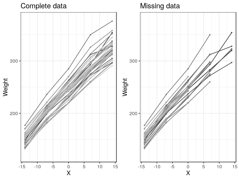
The data can be visualized as many lines, each representing a subject (rat).
p1 <- ggplot(d1, aes(x = X, y = RT, group = s, colour = s)) +
    geom_line(size = 1) +
    geom_point() + ylab("Weight") +
    ggtitle("Complete data") +
    coord_cartesian(ylim = c(120, 380)) +
    scale_colour_grey(na.value = "black") +
    theme_bw(base_size = 20) +
    theme(legend.position = "none")
Set-up Model
The DDM composes of two complementary defective distribtions; thereby, two response types. Unlike the DDM, a regression model has only one response type; that is one (complete) distribution. Therefore, the match.map and responses arguments are set as NULL and “r1” (meaning only one response type).
The argument regressors enters the independent / predictive variable (typically denoted X). In the Rats example, the weights of thirty young rats were measured weekly for five weeks and the measurements taken at the end of each week (8th, 15th, 22rd, 29th, & 36th day) were provided. The parameterization is a (intercept), b (slope) and the precision (\(= 1/sd^2\)).
require(ggdmc)
model <- BuildModel(
    p.map      = list(a = "1", b = "1", tau = "1"),
    match.map  = NULL,
    regressors = c(8, 15, 22, 29, 36) - tmp$xbar,,
    factors    = list(S = c("x1")),
    responses  = "r1",
    constants  = NULL,
    type       = "glm")
## Parameter vector names are: ( see attr(,"p.vector") )
## [1] "a"   "b"   "tau"
##
## Constants are (see attr(,"constants") ):
## NULL
##
## Model type = glm
Recovery Study
I take values from the Rats example as the true parameters at the population level and use them to simulate an ideal data set, which has 1000 rats and each of them contributes 100 response. tnorm2 is truncated normal distribution, using mean and precision parametrization. When both the upper and lower are set NA, the tnorm becomes normal distribution.
npar <- length(GetPNames(model))
pop.location  <- c(a = 242.7, b = 6.189, tau = .03)
pop.scale <- c(a = .005, b = 3.879, tau = .04)
ntrial <- 100
pop.prior  <-BuildPrior(
   dists = rep("tnorm2", npar),
   p1    = pop.location,
   p2    = pop.scale,
   lower = c(NA, 0, 0),
   upper = rep(NA, npar))
dat <- simulate(model, nsub = 1000, nsim = ntrial, prior = pop.prior)
dmi <- BuildDMI(dat, model)
ps  <- attr(dat, "parameters") ## Extract true parameters for each individual
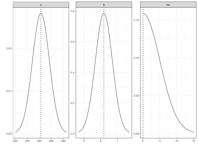
This plots the distributions that generate the simulation data and shows the location parameters of these distributions as dashed lines.
plot(pop.prior, ps = pop.mean)
Set up Priors
To randomly draw initial values for the data- and hyper-level parameters, I set up three sets of distributions and bind them as a list, named start. These are used to generate start values only.
pstart <- BuildPrior(
    dists = c("tnorm", "tnorm", "tnorm"),
    p1    = c(a = 242,  b = 6.19, tau = .027),
    p2    = c(a = 14, b = .49, tau = 10),
    lower = c(NA, NA, 0),
    upper = rep(NA, npar))
lstart <- BuildPrior(
    dists = c("tnorm", "tnorm", "tnorm"),
    p1    = c(a = 200,  b = 5, tau = .01),
    p2    = c(a = 50, b = 1, tau = .01),
    lower = c(NA, NA, 0),
    upper = rep(NA, npar))
sstart <- BuildPrior(
    dists = c("tnorm", "tnorm", "tnorm"),
    p1    = c(a = 10,  b = .5, tau = .01),
    p2    = c(a = 5, b = .1, tau = .01),
    lower = c(NA, NA, 0),
    upper = rep(NA, npar))
start <- list(pstart, lstart, sstart)
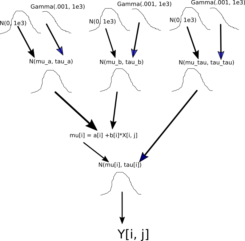
Next, I set up the structure of the hierarchical model. It is important to understand the hierarchical structure, so I sketch a diagram to show how the codes of setting up the prior distributions associate with the model structure.
p.prior  <- BuildPrior(
    dists = rep("tnorm2", npar),
    p1    = c(a = NA, b = NA, tau = NA),  ## the value are drawn from hyper-level
    p2    = rep(NA, 3),                   ## (mu and sigma) prior, so all set NA
    lower = c(NA, 0, 0),
    upper = rep(NA, npar))
mu.prior  <- BuildPrior(
    dists = rep("tnorm2", npar),
    p1    = c(a = 200, b = 6, tau = 3)
	p2    = c(a = 1e-4, b = 1e-3, tau = 1e-2)
    lower = c(NA, 0, 0),
    upper = rep(NA, npar))
sigma.prior <- BuildPrior(
    dists = rep("gamma", npar),
    p1    = c(a = .01, b = .01, tau = .01),
    p2    = c(a = 1000,  b = 1000, tau = 1000),
    lower = c(0, 0, 0),
    upper = rep(NA, npar))
prior <- list(p.prior, mu.prior, sigma.prior)
Sampling
The function, StartNewhiersamples use the start priors only for drawing initial values. The prior distributions wil be used in the model fit.
fit <- run(StartNewhiersamples(5e2, dmi, start, prior))
fit <- run(RestartHypersamples(5e2, fit, thin = 32))
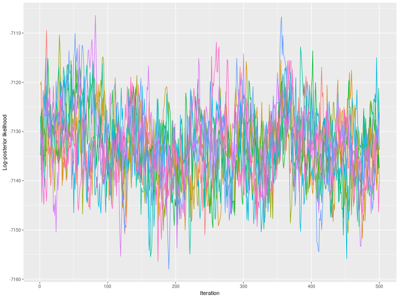
Model Diagnosis
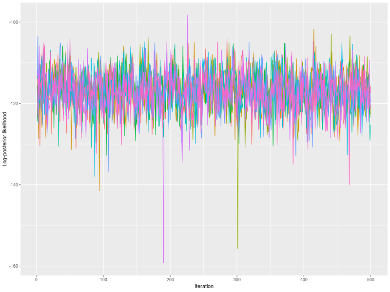
As usually, I check the potential scale reduction factors (Brook & Gelman,1998), effective sample sizes, and trace plots.
rhat <- hgelman(fit, verbose = TRUE)
hes <- effectiveSize(hsam, hyper = TRUE)
es1 <- effectiveSize(hsam[[1]])

##    a.h1     b.h1   tau.h1     a.h2     b.h2   tau.h2
## 427.9587 767.7925 483.1228 613.3212 730.1198 462.4242
##        a        b      tau
## 569.3685 609.0303 572.1573

p0 <- plot(fit, hyper = TRUE)
p1 <- plot(fit, hyper = TRUE, pll = FALSE, den = TRUE)
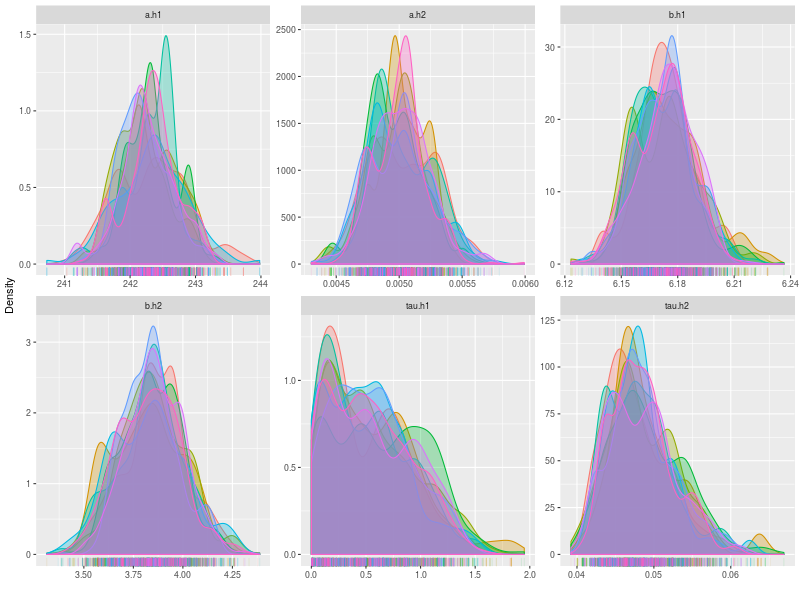
est1 <- summary(fit, hyper = TRUE, recover = TRUE, start = 101,
                ps = pop.mean,  type = 1, verbose = TRUE, digits = 3)
est2 <- summary(fit, hyper = TRUE, recover = TRUE, start = 101,
                ps = pop.scale, type = 2, verbose = TRUE, digits = 3)
est3 <- summary(fit, recover = TRUE, ps = ps, verbose = TRUE)

##                     a      b    tau
## True           242.700  6.189 0.030
## 2.5% Estimate  241.456  6.143 0.008
## 50% Estimate   242.275  6.173 0.460
## 97.5% Estimate 243.081  6.206 1.338
## Median-True     -0.425 -0.016 0.430
##
##                    a      b   tau
## True           0.005  3.879 0.040
## 2.5% Estimate  0.005  3.533 0.042
## 50% Estimate   0.005  3.835 0.047
## 97.5% Estimate 0.005  4.156 0.058
## Median-True    0.000 -0.044 0.007
##
## Summary each participant separately
##           a    b   tau
## Mean 242.28 6.17  3.82
## True 242.29 6.17  3.81
## Diff   0.01 0.00 -0.01
## Sd    14.14 0.51  2.80
## True  14.13 0.51  2.91
## Diff   0.00 0.00  0.11
Model Fit to Rats Data
After verifying that the model structure is OK, I then fit the Rats data.
## Each rat contribute 5 trials / observations
DT <- data.table(d)
DT[, .N, .(s)]
##      s N
##  1:  1 5
##  2:  2 5
##  3:  3 5
##  ...
## 30: 30 5
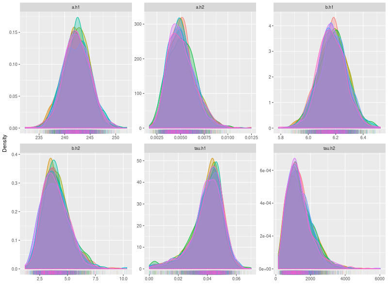
Now, I bind the Rats data with the model and start sampling. The estimates are fairly similar with BUGS and Stan estimations. The only significant difference is the tau.h1, which simply due the more complex structure used here.
dmi <- BuildDMI(d, model)
fit0 <- run(StartNewhiersamples(500, dmi, start, prior))
fit  <- run(RestartHypersamples(5e2, fit0, thin = 32))

est1 <- summary(fit, hyper = TRUE, type = 1, verbose = TRUE)
round( est1$quantiles, 3)
#              2.5%   25%     50%      75%  97.5%
# a.h1      237.37 240.69  242.49  244.12  247.75
# mu_alpha  237.09 240.68  242.47  244.29  247.84  ## Stan
# alpha.c   237.10 240.90  242.70  244.50  248.10  ## BUGS
# b.h1        5.98   6.10    6.17    6.24    6.37
# mu_beta     5.97   6.11    6.18    6.26    6.40  ## Stan
# beta.c      5.97   6.12    6.19    6.26    6.40  ## BUGS

# tau.h1     0.012  0.035   0.042   0.047   0.056
# Stan       0.020  0.024   0.027   0.030   0.036
# BUGS       0.020  0.024   0.027   0.030   0.036

# a.h2       0.003   0.004   0.005   0.006   0.008
# alpha.tau  0.003   0.004   0.005   0.006   0.008 ## BUGS
# b.h2       2.049   3.111   3.838   4.683   6.714
# beta.tau   1.952   3.078   3.879   4.922   8.026 ## BUGS

hes <- effectiveSize(fit, hyper = TRUE)
##     a.h1     b.h1   tau.h1     a.h2     b.h2   tau.h2
## 4500.000 4534.287 4193.927 3807.489 4079.768 3139.033

round(apply(data.frame(es), 1, mean))
round(apply(data.frame(es), 1, sd))
round(apply(data.frame(es), 1, max))
round(apply(data.frame(es), 1, min))
##         a    b  tau
## Mean 4464 4360 4321
## SD    139  242  348
## MAX  4717 5020 5137
## MIN  4100 3732 3455
Handling Missing Data
Rats example also considered fitting missing data. This can be done by setting the missing data as NA or downloading the missing data set directly from BUGS site.
d[6:10,5] <- NA
d[11:20,4:5] <- NA
d[21:25,3:5] <- NA
d[26:30,2:5] <- NA
and bind the data with the same model set up previously. Again, the results are fairly similar with using other Bayesian software.
dmi <- BuildDMI(d[!is.na(d$RT),], model)

  #            2.5%     25%    50%    75%     97.5%
  # a.h1     241.01  244.35  246.07  247.73  251.09
  # alpha.c  240.30  243.90  245.80  247.70  251.30 BUGS
  # b.h1      6.362   6.526   6.605   6.688   6.844
  # beta.c    6.286   6.477   6.572   6.669   6.870 BUGS
  # a.h2      0.003   0.004   0.005   0.006   0.009
  # alpha.tau 0.003   0.004   0.005   0.006   0.009 BUGS
  # b.h2      1.640   2.757   3.595   4.479   7.241
  # beta.tau  1.505   2.676   3.620   5.044  13.601 BUGS
The predictions for the final four observations on rat 26 can be obtained by entering predict_one function with fit[[26]].
pp26 <- predict_one(fit[[26]])
pred26 <- pp26[, .(Mean = mean(RT)), .(X)]
pred26[c(2,1,3,4,5),]

##      X     Mean
## 1: -14 160.8060
## 2:  -7 203.8068  Y[26, 2] = 204.6
## 3:   0 249.4786  Y[26, 3] = 250.2
## 4:   7 297.8309  Y[26, 4] = 295.6
## 5:  14 339.6564  Y[26, 5] = 341.2
Reference
Gelfand, A. E., Hills, S. E., Racine-Poon, A., & Smith, A. F. (1990). Illustration of Bayesian inference in normal data models using Gibbs sampling. Journal of the American Statistical Association, 85(412), 972-985.