This is a short note for doing least square minimization to fit a diffusion process model.

The aim of the least square minimization (LSM) is to minimize a cost function, which returns the difference between the data and model predictions.

One possible reason to fit data to a process model, instead of a standard model [e.g., ex-Wald, (Schwarz, 2001; Schwarz, 2002; Heathcote, 2004)] is to retain some flexibilities for later tweaking the process. A standard model usually has been thoroughtly studied, and thereby provides analytic likelihood functions. For example, one can find the analytic likelihood function of the drift-diffusion model in van Zandt (2000). (See, also e.g., equation (5) in Bogacz et al., 2006 for the standard stochastic process equation of the DDM).

The method of least square minimization is useful when one wants to test a number of differernt variants that deviate from the standard stochastic process. For instance, one might hypothesize that people deploy different drift rates to different regions in the visual field because people perhaps pay more attention to a more interesting centre region of a stimulus, than other regions. One could assign a larger mean drift rate to the centre region, comparing with assigning smaller mean drift rates to the others. Another possible hypothetical variant is that one might assume within a trial, people change their drift rate significantly (not just small variation due to within-trial variability). This could be tested by tweaking the standrd diffusion process, such as, constructing a series of different Gaussian models, each of which sample different drift rates at different time point in a process.

Nevertheless, one must note that the more variants one introduces to a process model that deviates from the standard process, the more likely that the altered process becomes difficult to fit (as well as prone to overfit the data).

Only a handful of process models, for example the full drift-diffusion model (DDM; see e.g., the Appendix in Van Zandt, 2000 for its PDF and CDF), have derived their analytic likelihood functions. After tweaking a standard process, one must also derive a new probability density function (PDF; sometimes as well as CDF) based on the altered new process. (See the video provided by StatQuesta for an excellent explantion regarding the probability and the likelihood at https://www.youtube.com/watch?v=pYxNSUDSFH4).). The process of deriving a new likelihood function could be sometimes cumbersome, if not very difficult or impossible. This of course assumes that one wants to apply the model fitting methods using likelihood functions. One advantage of deriving the analytic solution for a process model is that one can use the powerful maximum likelihood method to conduct model fitting.

On the other hand, the LSM, often used in machine learning, is one method for model fitting, without using the likelihood function.

The following code snippet is an R programme for a 1-D diffusion (process) model. The code snippet is to demonstrate how the process model is constructed. The real working programme is written in C++.

I assumed a within-trial constant (mean) drift rate as in a typical case of diffusion process. See code comments to get further details.

r1d_R <- function(pvec, tmax, h)
{
  ## p.vector <- c(v=0, a=1, z=.5, t0=0, s=1)
  Tvec <- seq(0, tmax, h)
  nmax <- length(Tvec)
  
  ## Unit travelling distance; ie how far a particle travels per unit time 
  ## 1. Here I used h (presumably to 1 ms) as the unit time
  ## 2. In the constant-drift model, the mean drift rate does not change 
  ##    within a process, although it is subjected to the influence of 
  ##    within-trial standard deviation (variability). That is, 
  ##    the "constant" refers to the mean drift rate is constant.
  ## 3. travel distance = drift rate * unit time 
  ##    the following one vector ( ie rep(1, nmax) ) is to make "mut" a 
  ##    vector. This pre-calculation helps to reduce computation time.
  mut <- h * pvec[1] * rep(1, nmax)
  
  ## - Within-trial standard deviation, 
  ## - The fifth element of pvec is the within-trial standard deviation
  sigma_wt <- sqrt(h) * pvec[5] * rnorm(nmax) 
  
  ## - Xt stores evidence values; 
  ## - To plot the trace of a particle, one can return Xt.
  ## - Xt is the assumed input (ie 'features' in ML terminology).
  ## - In EAM, we assume Xt is due to neuronal responses to sensory stimuli.
  ##   Thus, Xt is often called sensory evidence
  Xt <- rep(NA, nmax)
  
  ## - The first value for the evidnece vector is the assumed starting point
  ## - pvec[3] is the absolute value of the starting point.
  ## - If one wants to limit the process to a symmetric process, uncomment 
  ## the following line
  ## Xt[1] <- pvec[3] * pvec[2]  ## assume pvec[3] is zr and convert it to z.
  Xt[1] <- pvec[3]               ## assume pvec[3] is z
  current_evidence <- Xt[1];     ## transient storage for the evidence
  
  ## Start the evidence accumulation process
  ## Note 1. We did not know when the process would stop beforehand
  ## Note 2. We assumed the studied process cannot exceed nmax * h seconds
  ## Note 3. Only when the latest evidence value exceeds the threshold value,
  ##         a or 0, the process stops.
  i <- 2     ## starting from i == 2
  
  ## - pvec[2] is the upper boundary; 
  ## - 0 is the lower boundary.
  while (current_evidence < pvec[2] && current_evidence > 0 && i < nmax)
  {
    ## This is the typical diffusion process equation
    ## the updated evidence value = the latest evidence value + 
    ##    (drift rate * unit time) + within-trial standard deviation 
    Xt[i] <- Xt[i-1] + mut[i] + sigma_wt[i] 
    current_evidence <- Xt[i];  ## Store the updated evidence value 
    i <- i + 1;  ## increment step 
  }
  
  RT <- i * h + pvec[4];   ## decision time + t0 = response time 
  is_broken <- i == nmax;  ## whether the simulation suppasses the assumed max time 
  
  ## hit upper bound (1) or lower bound (0)
  R <- ifelse(current_evidence > pvec[2], 1, 0) 
  
  ## I use an R list to return extra information.
  return(list(Xt = Xt, Tvec= Tvec, RT=RT, R = R, is_broken=is_broken))
}

Simulate a Diffusion Process

To inspect an instance of a diffusion process, I designated a parameter vector and considered it as a “true” parameter vector.

This is just to conduct the simulation. In a regular model fitting, one would not know the true values of the parameters. One aim of fitting a model to data is to find a set optimal parameters describing the data.

I assumed a two-second time span for the diffusion process.

tmax <- 2
h <- 1e-3
p.vector <- c(v=0, a=1, z=.5, t0=0, s=1)
res1 <- r1d_R(pvec=p.vector, tmax=tmax, h=h)

## To locate the first instance of NA
idx <- sum(!is.na(res1$Xt)); 

plot(res1$Tvec[1:idx], res1$Xt[1:idx], type='l', ylim=c(0, 1), xlab='DT (s)',
     ylab='Evidence')
abline(h=p.vector[2], lty='dotted', lwd=1.5)
abline(h=0, lty='dotted', lwd=1.5)
points(x=0, y=p.vector[3], col='red', cex =2)

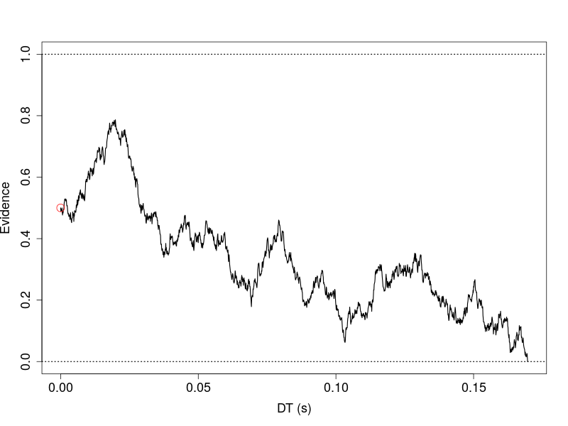
Usually, the instance represents or, said simulates, an unobservable cognitve process that happens when one responds to a stimulus. For example, in a driving simulation study, assuming the vehicle is automatically self-driving and a driver can decide to engage manually driving when needed. A participant sits in the simulator and meanwhile engages in some other tasks. The participant is instructed to make a decision to disengage the automatic driving, if, for example, a patch of simulated fog is unveiled and the front view shows a possible immediate collision with another vehicle(s).

One might assume the stimulus composes of the front vehicle, its surrondings, as well as the participant’s own kinetmatic sense of her/his vehicle (speed, accelaration etc), her/his assessment of the distance between her/his AV and the vehicle in the front.

The stimulus then presumably elicits some unobservable “sensory evidence”. The “sensory evidence” is the input (i.e., “Evidence” in the previous figure).

In a 2AFC diffusion model, the outputs usually are a pair of numbers. The most well-known is the response time (RT) and the other is response choice. The latter can be represented as 0 and 1 in a binary-choice task. The outputs are usually more easily to observe in a typical, standard psychological task. The input, however, is not.

Responses, Choices, and Accuracy

In a typical psychological task, participants respond by pressing pressing some keys via a device, such as customised key pad, a computer keyboard, a computer mouse, or a touch screen. For example, one can configure pressing “z” for option 1, and “/” for option 2. This action then is recorded for every response trial. Researchers then later infer which option participants have chosen in every single trial.

Note that participants may commit to choose option 1, (or option 2); however, a stimulus could belong to option 2 (or option 1). This is an outcome of mismatch. This brings us to the idea of matching responses to stimuli.

In other words, a response, in a binary task, could result in two different outcomes, correct or incorrect. For example in a two-choice lexical decision task, one would respond “word” or “non-word” to a stimuls, which could be real word (W) or a pesudo-word (NW).

Only after a response is committed has the outcome become apparent.

Table 1. A binary-choice stimulus-response table.

	W	NW
word	O	X
non-wrod	X	O

Objective Function

In the following, I presented a simple method to fit a two-choice diffusion model, using the LSM. First, I set up an objective function, which is designed to describe the difference between the model predictions and the data. As typically been done in the literature applying diffusion models, I compared the five percentils, .1, .3, .5, .7 and .9. I added error rates in the second model-fitting example. The following code snippet showed this calculation.

sq_diff <- c( (pred_q0 - data_q0)^2, (pred_q1 - data_q1)^2) 

To make the demonstration simple, I aimed only to recover the drift rate and fixed the other parameters (a, zr, t0, and s). I wrote another stand-alone C++ function, which simply used a for-loop wrap around the above r1d function and added a few checks on the data quality. I named this function, “rdiffusion”.

Next, the objective function took the drift rate parameter from the optimization routine and put it in the first position of the “pvec” object. I fixed the second to fifth parameters by manually entering their values. The objective function then simulated “nsim” number of diffusion processes. I passed 10,000 to the nsim object.

nsim <- 1e4

Then, I removed the outlier trials, storing their indices into the “bad” object. I designated NA to those process suppassing the assumed upper time limit (i.e., tmax). I also designated 0 and 1, respectively, to the processes that result in hitting lower and upper boundaries. Thus, the line with, “pred_R == 1”, was to extract the indices for the simulated trials hitting the upper boundary.

The line, “upper_count <- sum(upper)” was to count how many simulated trials result in choice 1 (i.e., htting upper boundary). This was to gauge the wild parameter values at the early stage of optimzation. The optimization routine may cast some drift rate values, resulting in the process that produces no responses (i.e., outside the parameter space, under the assumptions).

    bad <- (is.na(tmp[,2])) || (tmp[,2] == 2)
    sim <- tmp[!bad, ]
    
    pred_RT <- sim[,1]
    pred_R  <- sim[,2]

    upper <- pred_R == 1
    lower <- pred_R == 0
    upper_count <- sum(upper)
    lower_count <- sum(lower)

Next, the objective function returns a very large number, 1e9, if the parameters resulting in abnormal diffusion processes. Otherwise, I separated the RTs for the choice 1 and choice 2, respectively, for the data and for the predictions and then compared their five percentiles. Finally, the sum of the differences was sent back to the optimization routine.

        data_RT <- data[,1]
        data_R  <- data[,2]
        d_upper <- data[,2] == 1
        d_lower <- data[,2] == 0
        RT_c0   <- data_RT[d_upper]
        RT_c1   <- data_RT[d_lower]

        pred_c0 <- pred_RT[upper]
        pred_c1 <- pred_RT[lower]
        
        pred_q0 <- quantile(pred_c0, probs = seq(.1, .9, .2))
        pred_q1 <- quantile(pred_c1, probs = seq(.1, .9, .2))
        
        data_q0 <- quantile(RT_c0, probs = seq(.1, .9, .2))
        data_q1 <- quantile(RT_c1, probs = seq(.1, .9, .2))
        sq_diff <- c( (pred_q0 - data_q0)^2, (pred_q1 - data_q1)^2)
        out <- sum(sq_diff)

The complete objective function is listed in the following code snippet.

objective_fun <- function(par, data, tmax, h, nsim) {
    pvec <- c(par[1], 1, .5, 0, 1)
    tmp <- rdiffusion(nsim, pvec, tmax, h)

    bad <- (is.na(tmp[,2])) || (tmp[,2] == 2)
    sim <- tmp[!bad, ]
    
    pred_RT <- sim[,1]
    pred_R  <- sim[,2]

    upper <- pred_R == 1
    lower <- pred_R == 0
    upper_count <- sum(upper)
    lower_count <- sum(lower)

    
    if (any(is.na(pred_R))) {
        ## return a very big value, so the algorithm throws out
        ## this parameter
        out <- 1e9   
    } else if ( is.na(sum(upper_count)) || is.na(sum(lower_count)) ) {
        ## return a very big value, so the algorithm throws out
        ## this parameter
        out <- 1e9
    } else {
        data_RT <- data[,1]
        data_R  <- data[,2]
        d_upper <- data[,2] == 1
        d_lower <- data[,2] == 0
        RT_c0   <- data_RT[d_upper]
        RT_c1   <- data_RT[d_lower]

        pred_c0 <- pred_RT[upper]
        pred_c1 <- pred_RT[lower]
        
        pred_q0 <- quantile(pred_c0, probs = seq(.1, .9, .2))
        pred_q1 <- quantile(pred_c1, probs = seq(.1, .9, .2))
        
        data_q0 <- quantile(RT_c0, probs = seq(.1, .9, .2))
        data_q1 <- quantile(RT_c1, probs = seq(.1, .9, .2))
        sq_diff <- c( (pred_q0 - data_q0)^2, (pred_q1 - data_q1)^2)
        out <- sum(sq_diff)
    }
    
  return(out)
}

I used the optimize routine to search the parameters. To make the estimation simple, I limited the range of estimation to 0 to 5. The optimize is for searching one dimension space. See ?optimize for further details. For higher dimension, one must use other optimization routines.

fit <- optimize(f=objective_fun, interval=c(0, 5), data = dat,
                tmax=tmax, h=h, nsim=nsim)

To estimate the variability, I used a simple resampling method, via the parallel routine, mclapply, to conduct 100 parameter-recovery studies.

doit <- function(p.vector, n, tmax, h, nsim)
{
    dat <- rdiffusion(n, p.vector, tmax, h)
    fit <- optimize(f=objective_fun, interval=c(0, 5), data = dat,
                    tmax=tmax, h=h, nsim=nsim)
    return(fit)
}

The following is the code snippet for launching the parameter-recovery studies..

## Assume the "real" process has the parameters, p.vector
## The aim is to recover the drift rate , 1.51
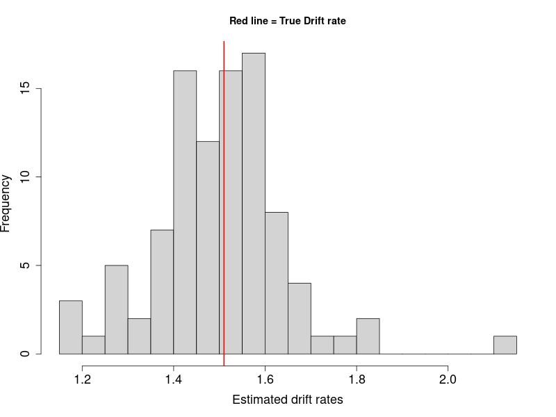
p.vector <- c(v=1.51, a=1, zr=.5, t0=0, s=1)
tmax  <- 2
h     <- 1e-3
ncore <- 3

## Assume we have collected "real" empirical data, which has 5,000 trials
n <- 5e3

## I requested the objective function to simulate 10,000 trials to 
## construct the simulated historgram, every time the optimization routine
## make a guess about what the drift rate could be.
nsim <- 1e4

## Each parallel thread run an independent parameter-recovery study. 
## Here I ran 100 separate parameter-recovery studies.

## About 5.24 mins on a very good CPU
parameters <- parallel::mclapply(1:100, function(i) try(doit(p.vector, n, tmax, h,
                                                            nsim), TRUE),
                                 mc.cores = getOption("mc.cores", ncore))

Results

The figure showed most estimated drift rates are around the true value (red line), with a roughly normally distributed shape.

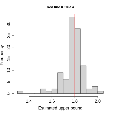
Recovering the Boundary Separation

To recover the parameter of boundary separation, I added the error rate statistics in the cost function. Moverover, I add a normalization factor, becaues the error rate and the RT percentiles are on different scales.

mymean <- function(x=NULL, nozero=0)
{
  ## A function from Bogacz and Cohen (2004)
    if(is.null(x)) {
      out <- 1
    } else {
      out <- ifelse(mean(x)==0 && nozero, 1, mean(x))
    }
    return(out)
}


doit <- function(p.vector, n, tmax, h, nsim)
{
    tmp <- rdiffusion(n, p.vector, tmax, h)
    tmp <- tmp[!is.na(tmp[,2]), ]
    tmp <- tmp[!is.na(tmp[,1]), ]
    over_tmax <- tmp[,2] == 2
    dat <- tmp[!over_tmax, ]
    fit <- subplex(par = runif(1), fn = objective_fun, hessian = FALSE,
                   data = dat, tmax=tmax, h=h, nsim=nsim)
    return(fit)
}

objective_fun <- function(par, data, tmax, h, nsim) {
    pvec <- c(2.35, par, .75, 0, 1)
    tmp <- rdiffusion(nsim, pvec, tmax, h)
    tmp <- tmp[!is.na(tmp[,2]), ]
    tmp <- tmp[!is.na(tmp[,1]), ]
    over_tmax <- tmp[,2] == 2
    sim <- tmp[!over_tmax, ]
    
    pred_RT <- sim[,1]
    pred_R  <- sim[,2]

    upper <- pred_R == 1
    lower <- pred_R == 0
    upper_count <- sum(upper)
    lower_count <- sum(lower)
    
    if ( (any(is.na(pred_R))) || is.na(sum(upper_count)) ||
         is.na(sum(lower_count)) || (length(pred_RT) == 0) ) {
        error <- 1e9
    } else {
        data_RT <- data[,1]
        data_R  <- data[,2]
        d_upper <- data[,2] == 1
        d_lower <- data[,2] == 0
        RT_c0   <- data_RT[d_upper]
        RT_c1   <- data_RT[d_lower]

        data_er <- 1 - mean(data_R)
        pred_er <- 1 - mean(pred_R)
        
        pred_c0 <- pred_RT[upper]
        pred_c1 <- pred_RT[lower]
        
        pred_q0 <- quantile(pred_c0, probs = seq(.1, .9, .2))
        pred_q1 <- quantile(pred_c1, probs = seq(.1, .9, .2))
        data_q0 <- quantile(RT_c0, probs = seq(.1, .9, .2))
        data_q1 <- quantile(RT_c1, probs = seq(.1, .9, .2))

        error <- sum( (data_q0 - pred_q0)^2 / mymean(data_q0, 1)^2 ) +
                 sum( (data_q1 - pred_q1)^2 / mymean(data_q1, 1)^2 ) +
            sum( (data_er - pred_er)^2 / mymean(data_er)^2 )
    }
  return(error)
}

This time I used a different optimization routine, subplex (Rowan, 1990).

tmax <- 2
h <- 1e-3
n <- 1e3    ## Assumed number of data points
p.vector <- c(v=2.35, a=1.8, z=.75, t0=0, s=1)  ## True values
nsim <- 1e4  ## number of model simulation
ncore <- 3

## 3176.639 s
parameters <- parallel::mclapply(1:100, function(i) 
              try(doit(p.vector, n, tmax, h, nsim), TRUE),
                       mc.cores = getOption("mc.cores", ncore))
save(parameters, p.vector, file = "data/fit_one_a.RData")

Results

The figure showed estimates distributed around the true value, 1.8 (red line).

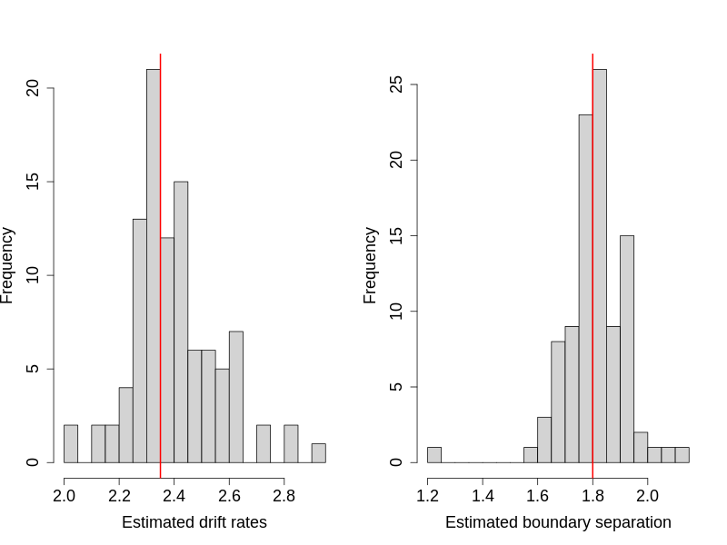
Recovering More Than One Parameter

Searching high-dimensional space might take substantial amount of time, but the computer codes essentially do not change too much. A parameter-recovery study to recover both the drift rate and the boundary separation took about 93 minutes, using a high-end CPU (2020)

Next

To fit empirical data, one must adjust the difference in time units in the model and experiment. The above model assumed a time unit, h, which is part of the model assumption. To fit empirical data, one must check whether this assumption is plausible and perhaps adjust accordingly.