Disclaimer: We have striven to minimize the number of errors. However, we cannot guarantee the note is 100% accurate. This note records the codes for fitting fixed-effect 2-D diffusion model.
In this tutorial, we conducted a parameter recovery of a CDDM associating a speed-and-accuracy (SAT) factor with the threshold parameter, a. A classic SAT experiment usually encourages participants to emphaize response speed in one condition and response accuracy in the other. The SAT factor is often found selectively affecting threshold-related parameters in 1-D diffusion model.
The model description prepares for a design with two factors: a three-level stimulus factor (S) and a two-level speed-and-accuracy (SAT) factor. However, it assumes only the threshold parameter, a is affected by the SAT factor and the S factor is inconseuqntial.
## This cleans up objects in the workspace, but already-loaded pacakges will be
## stilled loaded. To get a clear start of an R session, use the hot-key Ctrl-Shift-F10
## in RStudio for instance.
rm(list = ls())
require(ggdmc)

nw <- 4
model <- BuildModel(
  p.map     = list(v1 = "1", v2 = "1", a = "SAT", t0 = "1", sigma1="1",
                   sigma2="1", eta1="1", eta2="1", tmax="1", h="1"),
  match.map = NULL,
  constants = c(sigma1 = 1, sigma2 = 1, eta1=0, eta2=0, tmax=3, h=1e-4),
  factors   = list(S = c("s1", "s2", "s3"), SAT=c("speed", "accuracy")),
  responses = paste0('theta_', letters[1:nw]),
  type      = "cddm")
npar <- length(GetPNames(model))
In the following, we set up an assumed mechanism to generate twelve sets of true parameters, inside the simulate function. The true parameters are stored as a ps matrix, an attribute attached to the output object from the simulate function. Each row of the ps matrix represents one participant.
pop.mean  <- c(v1=1.2, v2=2.2, a.speed = 1.5, a.accuracy = 2.0, t0=0.1)
pop.scale <- c(v1=2.5, v2=2.5, a.speed=2,     a.accuracy=2.0,   t0=0.5)

pop.prior <- BuildPrior(
  dists = rep("tnorm", npar),
  p1    = pop.mean,
  p2    = pop.scale,
  lower = c(rep(-5, 2), 0, 0, 0),
  upper = c(rep( 5, 2), 5, 5, 2))


dat <- simulate(model, nsub=12, nsim = 30, prior = pop.prior);
ps  <- attr(dat, "parameters")
dmi <- BuildDMI(dat, model)
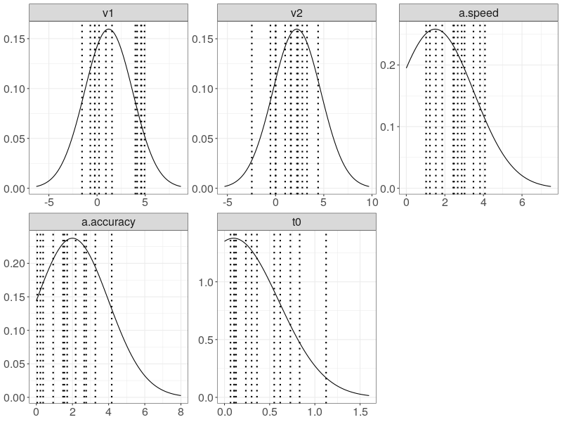
We then set up prior distributions for each CDDM parameter. Before we proceed to fit the data, we check whether our prior distributions cover the all true target parameters.
p.prior <- BuildPrior(
  dists = rep("tnorm", npar),
  p1    = pop.mean,
  p2    = pop.scale,
  lower = c(rep(-10, 2), 0, 0, 0),
  upper = c(rep( 10, 2), 8, 8, 5))

prior_d <- plot(p.prior, save = TRUE)

wide <- data.table::data.table(ps)
wide$s <- factor(1:nrow(ps))
pveclines <- data.table::melt.data.table(
  wide, id.vars = "s", variable.name = "Parameter", value.name = "true")

## require(ggplot2)
p0 <- ggplot(prior_d, aes_string(x = "xpos", y = "ypos")) +
  geom_line() +
  geom_vline(data = pveclines, aes_string(xintercept = "true"),
             linetype = "dotted", size = 1) +
  xlab("")+ ylab("")+
  facet_wrap(~Parameter, scales="free") +
  theme_bw() +
  theme(legend.position = "none",
        strip.text.x = element_text(size = 16),
        strip.text.y = element_blank(),
        axis.title.y = element_blank(),
        axis.text.x = element_text(size = 16),
        axis.text.y = element_text(size = 16),
        axis.title.x = element_blank())
Then we use 3 CPU cores, ncore=3 to run 3 parallel model fits. The block option indicates whether we want to update the entire parameter vector or just one parameter in the vector at a time. This is critical for the hierarchical model fit, but inconsequential for the fixed-effect model fit, so to gain more speed, we choose to disable it, block=FALSE.
Note in R 3.6.1, the mc.cores option in mclapply has been altered. It now takes the ncore option via “getOpion(“mc.cores”, 2L)”. This renders the ggdmc 0.2.6.0 always run 2 cores, which is a default setting of the mclapply function. To launch the number of CPU core you want, you have to adjust this manually in the two internal R functions, run_many and rerun_many, accordingly, or update your ggdmc via devtool tools.
## The latest ggdmc 0.2.7.1 will report its processing time!
## Processing time: 214.3 secs.
fit0 <- StartNewsamples(dmi, p.prior, block=FALSE, ncore=3)

## Processing time: 611.43 secs.
fit  <- run(fit0, block=FALSE, ncore=3)
After finishing the model fit, we check whether the chains are converged. The potential scale reduction factors, PSRT, are all below well 1.10.
rhat <- gelman(fit, verbose=TRUE)
# Diagnosing theta for many participants separately
# Mean    5    3   10    7    1    4    2   11    8   12    6    9
# 1.02 1.01 1.01 1.01 1.01 1.01 1.01 1.01 1.02 1.02 1.02 1.03 1.10

est <- summary(fit, recovery = TRUE, ps = ps, verbose = FALSE)
Plus, the parameters are precisely recovered.
# Summary each participant separately
#         v1    v2     a   t0
# Mean  1.98  1.92  1.52 0.12
# True  1.98  2.01  1.49 0.12
# Diff  0.00  0.10 -0.03 0.00
# Sd    0.14  0.17  0.12 0.04
# True  0.08  0.09  0.07 0.04
# Diff -0.06 -0.08 -0.05 0.00