Fixed-effects models assume each participant has his/her own specific mechanism of parameter generation. This assumption is relative to the random-effect models, which assume one common mechanism is responsible for generating parameters for all participants. The latter is sometimes dubbed, hierarchical or multi-level models, although the three terms could carry subtle different ideas.
In this tutorial, I illustrated the method of conducting the fixed-effects modelling. Given many observations of response times (RT) and choices, one modelling aim is to estimate the parameters that generate the observations.
A typical scenario is we collect data by inviting participants to visit our laboratory, having them do some cognitive tasks, and recording their RTs and choices.
Often, we would use a RT model, for example diffusion decision model (DDM) (Ratcliff & McKoon, 2008)1 to estimate latent variables. I first set up a model object. The type = “rd”, refers to Ratcliff’s diffusion model.
require(ggdmc)
model <- BuildModel(
  p.map     = list(a = "1", v = "1", z = "1", d = "1", sz = "1", sv = "1",
                   t0 = "1", st0 = "1"),
  match.map = list(M = list(s1 = "r1", s2 = "r2")),
  factors   = list(S = c("s1", "s2")),
  responses = c("r1", "r2"),
  constants = c(st0 = 0, d = 0),
  type      = "rd")

p.vector <- c(a = 1, v = 1.2, z = .38, sz = .25, sv = .2, t0 = .15)
ntrial <- 1e2
dat <- simulate(model, nsim = ntrial, ps = p.vector)
dmi <- BuildDMI(dat, model)
## A tibble: 200 x 3     ## use dplyr::tbl_df(dat) to print this
##    S     R        RT
##    <fct> <fct> <dbl>
##  1 s1    r1    0.249
##  2 s1    r1    0.246
##  3 s1    r2    0.262
##  4 s1    r1    0.519
##  5 s1    r1    0.205
##  6 s1    r1    0.177
##  7 s1    r1    0.174
##  8 s1    r1    0.378
##  9 s1    r1    0.197
## 10 s1    r1    0.224
##  ... with 190 more rows
Because the data were simulated from one set of presumed true values, p.vector, I can use them later to verify whether the sampling process does recovery the parameters. In Bayesian inference, we also need prior distributions, so let’s build a set of prior distributions for each DDM parameters.
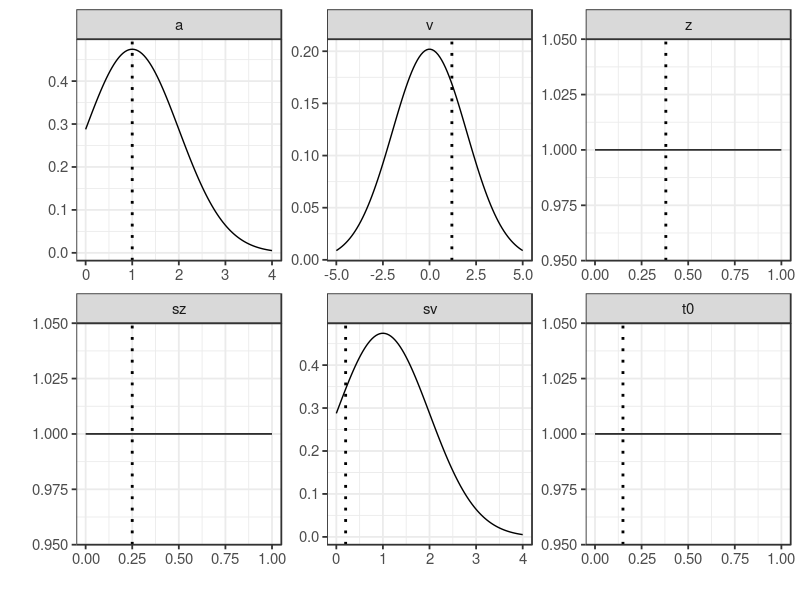
A beta distribution with shape1 = 1 and shape2 = 1, equals to a uniform distribution (beta(1, 1)). This choice was to regularize the parameters, (1) the start point, z, (2) its variability sz and (3) t0. All three were bounded by 0 and 1. Others used truncated normal distributions bounded by lower and upper arguments.
plot drew the prior distributions, providing a visual check method. This method, in the case of parameter recovery study, was to make sure the prior distribution does cover the true values.
p.prior  <- BuildPrior(
  dists = c(rep("tnorm", 2), "beta", "beta", "tnorm", "beta"),
  p1    = c(a = 1, v = 0, z = 1, sz = 1, sv = 1, t0 = 1),
  p2    = c(a = 1, v = 2, z = 1, sz = 1, sv = 1, t0 = 1),
  lower = c(0, -5, NA, NA, 0, NA),
  upper = c(5,  5, NA, NA, 5, NA))
plot(p.prior, ps = p.vector)
By default StartNewsamples used p.prior to randomly draw start points and samples 200 MCMC samples. This step used a mixture of crossover and migration operators. The run function by default drew 500 MCMC samples, using only crossover operator. gelman function reported PSRF value of 1.06 in this case. A potential scale reduction factor (PSRF2) less than 1.1 suggested chains are converged.
fit0 <- StartNewsamples(dmi, p.prior)
fit  <- run(fit0)
rhat <- gelman(fit, verbose = TRUE)
es   <- effectiveSize(fit)
## Diagnosing a single participant, theta. Rhat = 1.06
plot by default drew posterior log-likelihood. With the option, start, it changed to a latter start iteration to draw.
p0 <- plot(fit0)
## p0 <- plot(fit0, start = 101)
p1 <- plot(fit)

png("pll.png", 800, 600)
gridExtra::grid.arrange(p0, p1, ncol = 1)
dev.off()
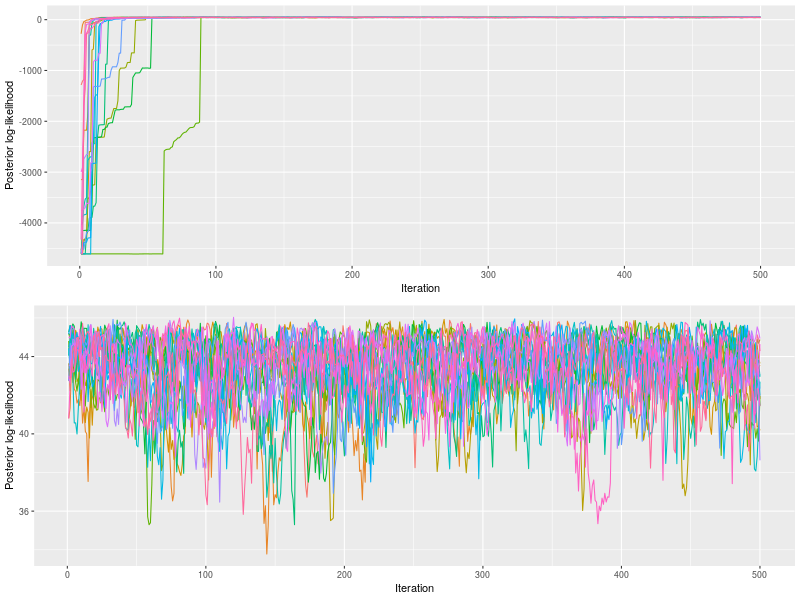
The upper panel showed the chains quickly converged to posterior log-likelihoods near 100th iteration and the bottom panel confirmed the rhat value (< 1.1).
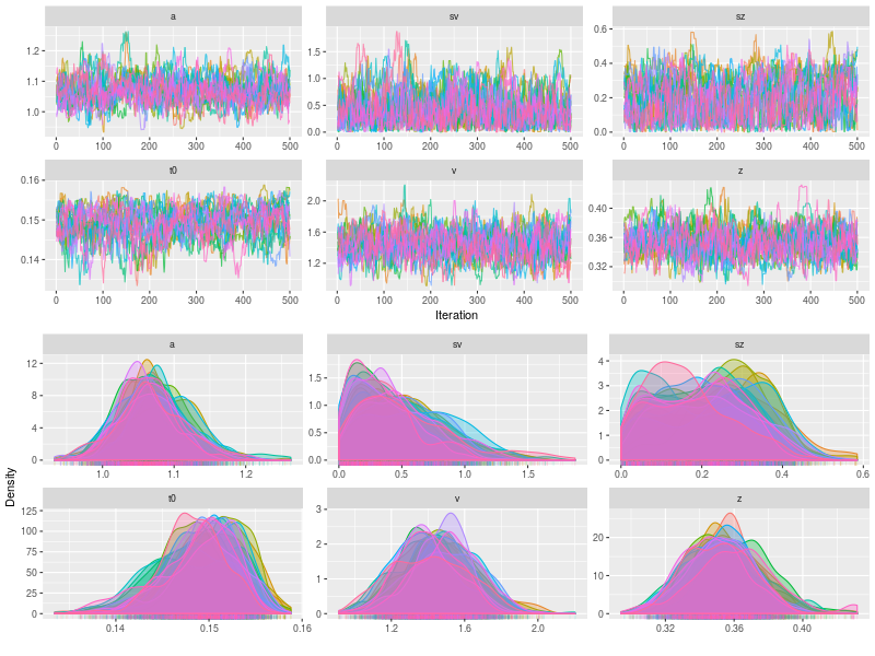
p2 <- plot(fit, pll = FALSE, den= FALSE)
p3 <- plot(fit, pll = FALSE, den= TRUE)
png("den.png", 800, 600)
gridExtra::grid.arrange(p2, p3, ncol = 1)
dev.off()
In a simulation study, we can check whether the sampling process is OK, using summary
est <- summary(fit, recover = TRUE, ps = p.vector, verbose = TRUE)
## Recovery summarises only default quantiles: 2.5% 50% 97.5%
##                     a     sv      sz      t0      v     z
## True           1.0000 0.2000  0.2500  0.1500 1.2000 0.3800
## 2.5% Estimate  0.9656 0.0401  0.0112  0.1338 1.1463 0.3504
## 50% Estimate   1.0419 0.6010  0.2174  0.1444 1.4983 0.3867
## 97.5% Estimate 1.1509 1.7128  0.4781  0.1522 2.0005 0.4273
## Median-True    0.0419 0.4010 -0.0326 -0.0056 0.2983 0.0067
Finally, we might want to check whether the model fits the data well. There are many methods to quantify the goodness of fit. Here, I illustrated two methods. First method is to calculate DIC and BPIC. These information criteria are useful for model selection. (need > ggdmc 2.5.5)
DIC(fit)
DIC(fit, BPIC=TRUE)
Secondly, I simulated post-predictive data. xlim trims off outlier values in the simulation. Note there are two different versions of the post-predictive functions, because the ggdmc version > 0.2.7.5 starts to use S4 class, which use @, instead of $ to extract elemnts in an object.
predict_one <- function(object, npost = 100, rand = TRUE, factors = NA,
                        xlim = NA, seed = NULL)
{
    require(ggdmc)
    if(packageVersion('ggdmc') == '0.2.6.0') {
        message('Using $ to extract object in v 0.2.6.0')
        out <- predict_one0260(object, npost, rand, factors, xlim, seed)
    } else {
        message('Using @ to extract object in v 0.2.6.0')
        out <- predict_one0280(object, npost, rand, factors, xlim, seed)
    }
    return(out)
}

predict_one0260 <- function(object, npost, rand, factors, xlim, seed)
{
  model <- attr(object$data, 'model')
  facs <- names(attr(model, "factors"));

  if (!is.null(factors))
  {
    if (any(is.na(factors))) factors <- facs
    if (!all(factors %in% facs))
      stop(paste("Factors argument must contain one or more of:", paste(facs, collapse=",")))
  }

  resp <- names(attr(model, "responses"))
  ns   <- table(object$data[,facs], dnn = facs)
  npar   <- object$n.pars
  nchain <- object$n.chains
  nmc    <- object$nmc
  ntsample <- nchain * nmc
  pnames   <- object$p.names
  thetas <- matrix(aperm(object$theta, c(3,2,1)), ncol = npar)

  colnames(thetas) <- pnames

  if (is.na(npost)) {
    use <- 1:ntsample
  } else {
    if (rand) {
      use <- sample(1:ntsample, npost, replace = F)
    } else {
      ## Debugging purpose
      use <- round(seq(1, ntsample, length.out = npost))
    }
  }

  npost  <- length(use)
  posts   <- thetas[use, ]
  nttrial <- sum(ns) ## number of total trials

  v <- lapply(1:npost, function(i) {
    ggdmc:::simulate_one(model, n = ns, ps = posts[i,], seed = seed)
  })

  out <- data.table::rbindlist(v)
  reps <- rep(1:npost, each = nttrial)
  out <- cbind(reps, out)

  if (!any(is.na(xlim)))
  {
    out <- out[RT > xlim[1] & RT < xlim[2]]
  }

  return(out)
}

predict_one0280 <- function(object, npost, rand, factors, xlim, seed)
{
    ## Update for using S4 class
    model <- object@dmi@model
    facs <- names(attr(model, "factors"));

    if (!is.null(factors))
    {
        if (any(is.na(factors))) factors <- facs
        if (!all(factors %in% facs))
            stop(paste("Factors argument must contain one or more of:", paste(facs, collapse=",")))
    }


    resp <- names(attr(model, "responses"));
    ns   <- table(object@dmi@data[,facs], dnn = facs);
    npar   <- object@npar
    nchain <- object@nchain
    nmc    <- object@nmc;
    ntsample <- nchain * nmc
    pnames   <- object@pnames

    thetas <- matrix(aperm(object@theta, c(3,2,1)), ncol = npar)
    colnames(thetas) <- pnames

  if (is.na(npost)) {
    use <- 1:ntsample
  } else {
    if (rand) {
      use <- sample(1:ntsample, npost, replace = F)
    } else {
	  ## Debugging purpose
      use <- round(seq(1, ntsample, length.out = npost))
    }
  }

  npost  <- length(use)
  posts   <- thetas[use, ]
  nttrial <- sum(ns) ## number of total trials

  v <- lapply(1:npost, function(i) {
    ggdmc:::simulate_one(model, n = ns, ps = posts[i,], seed = seed)
  })

  out <- data.table::rbindlist(v)
  reps <- rep(1:npost, each = nttrial)
  out <- cbind(reps, out)

  if (!any(is.na(xlim)))
  {
    out <- out[RT > xlim[1] & RT < xlim[2]]
  }

  return(out)
}


pp  <- predict_one(fit, xlim = c(0, 5))
dat <- fit@dmi@data  ## use this line for version > 0.2.7.5
## dat <- fit$data   ## use this line for version 0.2.6.0

dat$C <- ifelse(dat$S == "s1"  & dat$R == "r1",  TRUE,
         ifelse(dat$S == "s2" & dat$R == "r2", TRUE,
         ifelse(dat$S == "s1"  & dat$R == "r2", FALSE,
         ifelse(dat$S == "s2" & dat$R == "r1",  FALSE, NA))))
pp$C <- ifelse(pp$S == "s1"  & pp$R == "r1",  TRUE,
        ifelse(pp$S == "s2" & pp$R == "r2", TRUE,
        ifelse(pp$S == "s1"  & pp$R == "r2", FALSE,
        ifelse(pp$S == "s2" & pp$R == "r1",  FALSE, NA))))

dat$reps <- NA
dat$type <- "Data"
pp$reps <- factor(pp$reps)
pp$type <- "Simulation"

DT <- rbind(dat, pp)

require(ggplot2)
p1 <- ggplot(DT, aes(RT, color = reps, size = type)) +
  geom_freqpoly(binwidth = .05) +
  scale_size_manual(values = c(1, .3)) +
  scale_color_grey(na.value = "black") +
  theme(legend.position = "none") +
  facet_grid(S ~ C)
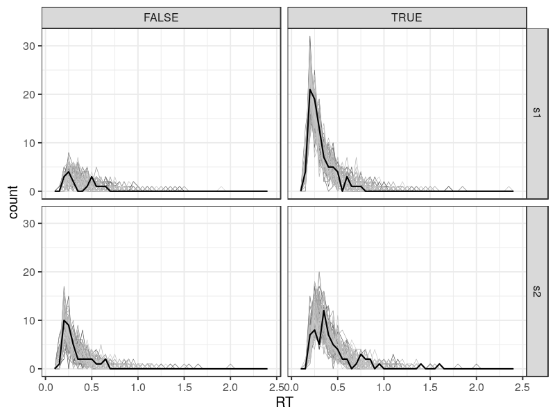
The grey lines are model predictions. By default, predict_one randomly draws 100 parameter estimates and simulate data based on them. Therefore, there are 100 lines, showing the prediction variability. The solid dark line shows the data. In this case, the dark line is within the range covering by the grey lines. Note that the error responses (FALSE) are not predicted as well as the correct responses. This is fairly common, when the number of trial is small. In this case, it has only 13 trials.